Using R: setting a colour scheme in ggplot2

Note to self: How to quickly set a colour scheme in ggplot2.

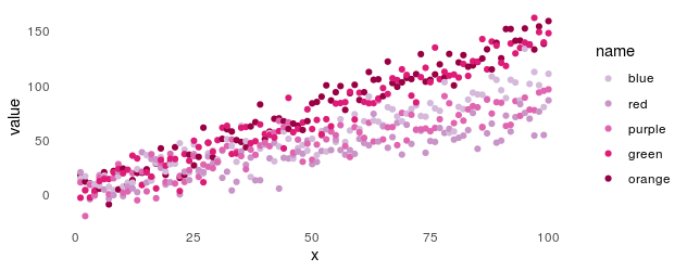
Imagine we have a series of plots that all need a uniform colour scale. The same category needs to have the same colour in all graphics, made possibly with different packages and by different people. Instead of hard-coding the colours and the order of categories, we can put them in a file, like so:

library(readr)
colours <- read_csv("scale_colours.csv")
# A tibble: 5 x 2
  name   colour 
      
1 blue   #d4b9da
2 red    #c994c7
3 purple #df65b0
4 green  #dd1c77
5 orange #980043

Now a plot with default colours, using some made-up data:

x <- 1:100

beta <- rnorm(5, 1, 0.5)

stroop <- data.frame(x,
                     sapply(beta, function(b) x * b + rnorm(100, 1, 10)))
colnames(stroop)[2:6] <- c("orange", "blue", "red", "purple", "green") 

data_long <- pivot_longer(stroop, -x)

plot_y <- qplot(x = x,
                y = value,
                colour = name,
                data = data_long) +
  theme_minimal() +
  theme(panel.grid = element_blank())

Now we can add the custom scale like this:

plot_y_colours <- plot_y + 
  scale_colour_manual(limits = colours$name,
                      values = colours$colour)


Using R: simple Gantt chart with ggplot2

Jeremy Yoder’s code for a simple Gantt chart on the Molecular Ecologist blog uses geom_line and gather to prepare the data structure. I like using geom_linerange and a coord_flip, which lets you use start and end columns directly without pivoting.

Here is a very serious data frame of activities:

# A tibble: 6 x 4
  activity       category        start               end                
                                                  
1 Clean house    preparations    2020-07-01 00:00:00 2020-07-03 00:00:00
2 Pack bags      preparations    2020-07-05 10:00:00 2020-07-05 17:00:00
3 Run to train   travel          2020-07-05 17:00:00 2020-07-05 17:15:00
4 Sleep on train travel          2020-07-05 17:15:00 2020-07-06 08:00:00
5 Procrastinate  procrastination 2020-07-01 00:00:00 2020-07-05 00:00:00
6 Sleep          vacation        2020-07-06 08:00:00 2020-07-09 00:00:00

And here is the code:


library(ggplot2)
library(readr)

activities <- read_csv("activities.csv")

## Set factor level to order the activities on the plot
activities$activity <- factor(activities$activity,
                              levels = activities$activity[nrow(activities):1])
    
plot_gantt <- qplot(ymin = start,
                    ymax = end,
                    x = activity,
                    colour = category,
                    geom = "linerange",
                    data = activities,
                    size = I(5)) +
    scale_colour_manual(values = c("black", "grey", "purple", "yellow")) +
    coord_flip() +
    theme_bw() +
    theme(panel.grid = element_blank()) +
    xlab("") +
    ylab("") +
    ggtitle("Vacation planning")

Using R: When weird errors occur in packages that used to work, check that you’re not feeding them a tibble

There are some things that are great about the tidyverse family of R packages and the style they encourage. There are also a few gotchas. Here’s a reminder to myself about this phenomenon: tidyverse-style data frames (”tibbles”) do not simplify to vectors upon extracting a single column with hard bracket indexing.

Because some packages rely on specific data.frame behaviours that tibbles don’t show, functions that work nicely with data frames, and normally have nice interpretable error messages, may mysteriously collapse in all kinds of ways when fed a tibble.

Here’s an example with MCMCglmm. This is not to pick on MCMCglmm; it just happened to be one of the handful of packages where I’ve run into this issue. Here, we use readr, the tidyverse alternative to the read.table family of functions to read some simulated data. The base function is called read.csv, and the readr alternative is read_csv.

Reading in tabular data is a surprisingly hard problem: tables can be formatted in any variety of obnoxious ways, and the reading function also needs to be fast enough to deal with large files. Using readr certainly isn’t always painless, but it reduces the friction a lot compared to read.table. One of the improvements is that read_csv will return a data.frame with the class tbl_df, affectionately called ”tibble

After reading the data, we centre and scale the trait, set up some priors and run an animal model. Unfortunately, MCMCglmm will choke on the tibble, and deliver a confusing error message.

library(MCMCglmm)
library(readr)

ped <- read_csv("sim_ped.csv")
pheno <- read_csv("sim_pheno.csv")

pheno$scaled <- scale(pheno$pheno)

prior_gamma <- list(R = list(V = 1, nu = 1),
                    G = list(G1 = list(V = 1, nu = 1)))

model <- MCMCglmm(scaled ~ 1,
                  random = ~ animal,
                  family = "gaussian",
                  prior = prior_gamma,
                  pedigree = ped,
                  data = pheno,
                  nitt = 100000,
                  burnin = 10000,
                  thin = 10)

Error in inverseA(pedigree = pedigree, scale = scale, nodes = nodes) : 
  individuals appearing as dams but not in pedigree
In addition: Warning message:
In if (attr(pedigree, "class") == "phylo") { :
  the condition has length > 1 and only the first element will be used

In this pedigree, it is not the case that there are individuals appearing as dams but not listed. If we turn the data and pedigree into vanilla data frames instead, it will work:

ped <- as.data.frame(ped)
pheno <- as.data.frame(pheno)

model <- MCMCglmm(scaled ~ 1,
                  random = ~ animal,
                  family = "gaussian",
                  prior = prior_gamma,
                  pedigree = ped,
                  data = pheno,
                  nitt = 100000,
                  burnin = 10000,
                  thin = 10)

                       MCMC iteration = 0

                       MCMC iteration = 1000

                       MCMC iteration = 2000