Toying with models: The Luria–Delbrück fluctuation test

I hope that Genetics will continue running expository papers about their old classics, like this one by Philip Meneely about Luria & Delbrück (1943). Luria & Delbrück performed an experiment on bacteriophage resistance in Escherichia coli, growing bacterial cultures, exposing them to a phage, and then plating and counting the survivors, who have become resistant to the phage. They considered two hypotheses: either resistance occurs adaptively, in response to the phage, or it occurs by mutation some time during the growth of the culture but before the phages are added. They find the latter to be the case, and this is an example of how mutations happen irrespective of their effects of fitness, in a sense at random. Their analysis is based on a model of bacterial growth and mutation, and the aim of this exercise is to explore this model by simulating some data.

First, we assume that mutation happens with a fixed mutation rate \mu = 2 \cdot 10^{-8} , which is quite close to their estimated value, and that the mutation can’t reverse. We also assume that the bacteria grow by doubling each generation up to 30 generations. We start a culture from a single susceptible bacterium, and let it grow for a number of generations before the phage is added. (We’re going to use discrete generations, while Luria & Delbrück use a continuous function.) Then:

n_{susceptible,i+1}= 2 (n_{susceptible,i} - n_{mutants,i})

n_{resistant,i+1} = 2 (n_{resistant,i} + n_{mutants,i})

That is, every generation i, the mutants that occur move from the susceptible to the resistant category. The number of mutants that happen among the susceptible is binomially distributed:

n_{mutants,i} \sim Binomial(n_{susceptible,i}, \mu) .

This is an R function to simulate a culture:

culture <- function(generations, mu) {
  n_susceptible <- numeric(generations)
  n_resistant <- numeric(generations)
  n_mutants <- numeric(generations)
  n_susceptible[1] <- 1
  for (i in 1:(generations - 1)) {
    n_mutants[i] <- rbinom(n = 1, size = n_susceptible[i], prob = mu)
    n_susceptible[i + 1] &lt;- 2 * (n_susceptible[i] - n_mutants[i])
    n_resistant[i + 1] &lt;- 2 * (n_resistant[i] + n_mutants[i])
  }
  data.frame(generation = 1:generations,
             n_susceptible,
             n_resistant,
             n_mutants)
}
cultures <- replicate(1000, culture(30, 2e-8), simplify = FALSE)

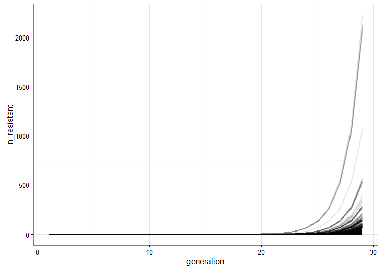
We run a few replicate cultures and plot the number of resistant bacteria. This graph shows the point pretty well: Because of random mutation and exponential growth, the cultures where mutations happen to arise relatively early will give rise to a lot more resistant bacteria than the ones were the first mutations are late. Therefore, there will be a lot of variation between the cultures because of their different histories.

resistant

combined <- Reduce(function (x, y) rbind(x, y), cultures)
combined$culture <- rep(1:1000, each = 30)

resistant_plot <- qplot(x = generation, y = n_resistant, group = culture,
      data = combined, geom = "line", alpha = I(1/10), size = I(1)) + theme_bw()

We compare this to what happens under the alternative hypothesis where resistance arises as a consequence of introduction of the phage with some resistance rate (this is not the same as the mutation rate above, even though we’re using the same value). Then the number of resistant cells in a culture will be: n_{acquired} \sim Binomial(2^{29}, \mu_{aquried}) .

resistant <- unlist(lapply(cultures, function(x) max(x$n_resistant)))

acquired_resistant <- rbinom(n = 1000, size = 2^29, 2e-8)

resistant_combined <- rbind(transform(data.frame(resistant = acquired_resistant), model = "acquired"),
                            transform(data.frame(resistant = resistant), model = "mutation"))

resistant_histograms <- qplot(x = resistant, data = resistant_combined,bins = 10) +
  facet_wrap(~ model, scale = "free_x")

histograms

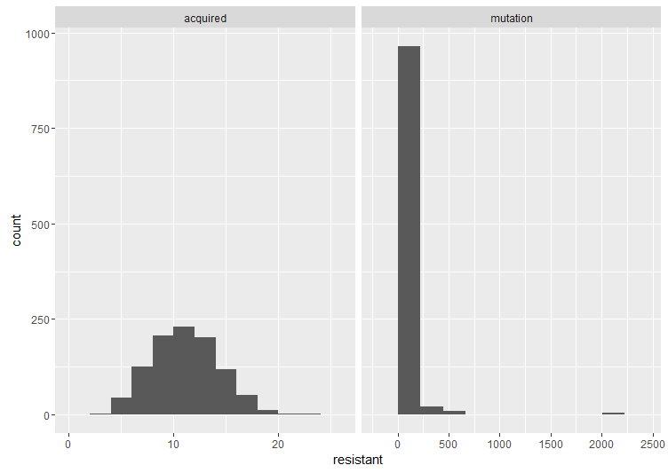
Here are two histograms side by side to compare the cases. The important thing is the shape. If the acquired resistance hypothesis holds, the number of resistant bacteria in replicate cultures follows a Poisson distribution, because it arises when one counts the number of binomially distributed events that occur in a given number of trials. The interesting thing about the Poisson distribution in this case is that its mean is equal to the variance. However, under the mutation model (as we’ve already illustrated), there is a lot of variation between cultures. These fluctuations make the variance much larger than the mean, which is also what Luria and Delbrück found in their data. Therefore, the results are inconsistent with acquired mutation, and hence the experiment is called the Luria–Delbrück fluctuation test.

mean(resistant)
var(resistant)
mean(acquired_resistant)
var(acquired_resistant)

Literature

Luria, S. E., & Delbrück, M. (1943). Mutations of bacteria from virus sensitivity to virus resistance. Genetics, 28(6), 491.

Meneely, P. M. (2016). Pick Your Poisson: An Educational Primer for Luria and Delbrück’s Classic Paper. Genetics, 202(2), 371-375.

Code on github.

Tre rekommendationer

1. Imre Lakatos, Science and pseudoscience

Vetenskapsfilosofi är något folk i allmänhet, och jag själv i synnerhet, borde läsa mer av och tänka mer på. Svårt verkar det också — trots käcka bilder och Richard Feynman-citat. Imre Lakatos var en vetenskapsfilosof vars namn jag stött på här och där, men inte läst något av förrän alldeles nyligen. Via Dynamic Ecology hittade jag en länk till ett av hans föredrag:

As opposed to Popper the methodology of scientific research programmes does not offer instant rationality. One must treat budding programmes leniently: programmes may take decades before they get off the ground and become empirically progressive. Criticism is not a Popperian quick kill, by refutation. Important criticism is always constructive: there is no refutation without a better theory. Kuhn is wrong in thinking that scientific revolutions are sudden, irrational changes in vision. … On close inspection both Popperian crucial experiments and Kuhnian revolutions turn out to be myths: what normally happens is that progressive research programmes replace degenerating ones.

2. Trudy Mackay, The genetic architecture of quantitative traits

Jag var på ESEB-konferensen i Lissabon i somras och det var helt fantastiskt på snart sagt alla sätt (mitt glada jollrande om konferensen finns här och här). Bland det bästa var det här föredraget från Trudy Mackay — en av dem som bokstavligen skrev boken om kvantitativ genetik.  Mackay pratade om hennes grupps arbete med genetisk kartläggning av kvantitativa egenskaper i bananflugor och om gen–gen-interaktioner, som det verkar finnas förvånansvärt många av — vilket gör saker mer komplicerade och roligare. Naturligtvis blir det ganska tekniskt efter hand och presentationsbilderna är tyvärr oläsliga, men det rekommenderas ändå varmt. Dessutom börjar Mackay med en genomgång av vad kvantitativ genetik är, varför det är viktigt och varför en kan lära sig så mycket från bananflugor. Det här är ett av mina favoritcitat:

Those of you who don’t work with flies might be surprised to learn that flies vary for any phenotype that an investigator has the imagination to develop a quantitative assay for.

Några fler föredrag från konferensen har publicerats och det kommer bli fler på ESEB2013:s YouTube-kanal.

3. Richard Lenski, Telliamed Revisited

Richard Lenski är evolutionsbiolog som förmodligen är mest känd för sitt Long Term Evolution Experiment — ett evolutionsexperiment med bakterien Escherichia coli. På sin blogg skriver han bland annat om vad de hittat i det experimentet — börja till exempel med den här posten:

Fitness is the central phenotype in evolutionary theory; it integrates and encapsulates the effects of all mutations and their resulting phenotypic changes on reproductive success.  Fitness depends, of course, on the environment, and here we measure fitness in the same medium and other conditions as used in the LTEE.  We estimate the mean fitness of a sample from a particular population at a particular generation by competing the sample against the ancestral strain, and we distinguish them based on a neutral genetic marker.  Prior to the competition, both competitors have been stored in a deep freezer, then revived, and acclimated separately for several generations before they are mixed to start the assay proper.  Fitness is calculated as the ratio of their realized growth rates as the ancestor and its descendants compete head-to-head under the conditions that prevailed for 500 … or 5000 … or 50,000 generations.