Journal club of one: ”Genomic predictions for crossbred dairy cattle”

A lot of dairy cattle is crossbred, but genomic evaluation is often done within breed. What about the crossbred individuals? This paper (VanRaden et al. 2020) describes the US Council on Dairy Cattle Breeding’s crossbred genomic prediction that started 2019.

In short, the method goes like this: They describe each crossbred individual in terms of their ”genomic breed composition”, get predictions for each them based on models from all the breeds separately, and then combine the results in proportion to the genomic breed composition. The paper describes how they estimate the genomic breed composition, and evaluated accuracy by predicting held-out new data from older data.

The genomic breed composition is a delightfully elegant hack: They treat ”how much breed X is this animal” as a series of traits and run a genomic evaluation on them. The training set: individuals from sets of reference breeds with their trait value set to 100% for the breed they belong to and 0% for other breeds. ”Marker effects for GBC [genomic breed composition] were then estimated using the same software as for all other traits.” Neat. After some adjustment, they can be interpreted as breed percentages, called ”base breed representation”.

As they already run genomic evaluations from each breed, they can take these marker effects and then animal’s genotypes, and get one estimate for each breed. Then they combine them, weighting by the base breed representation.

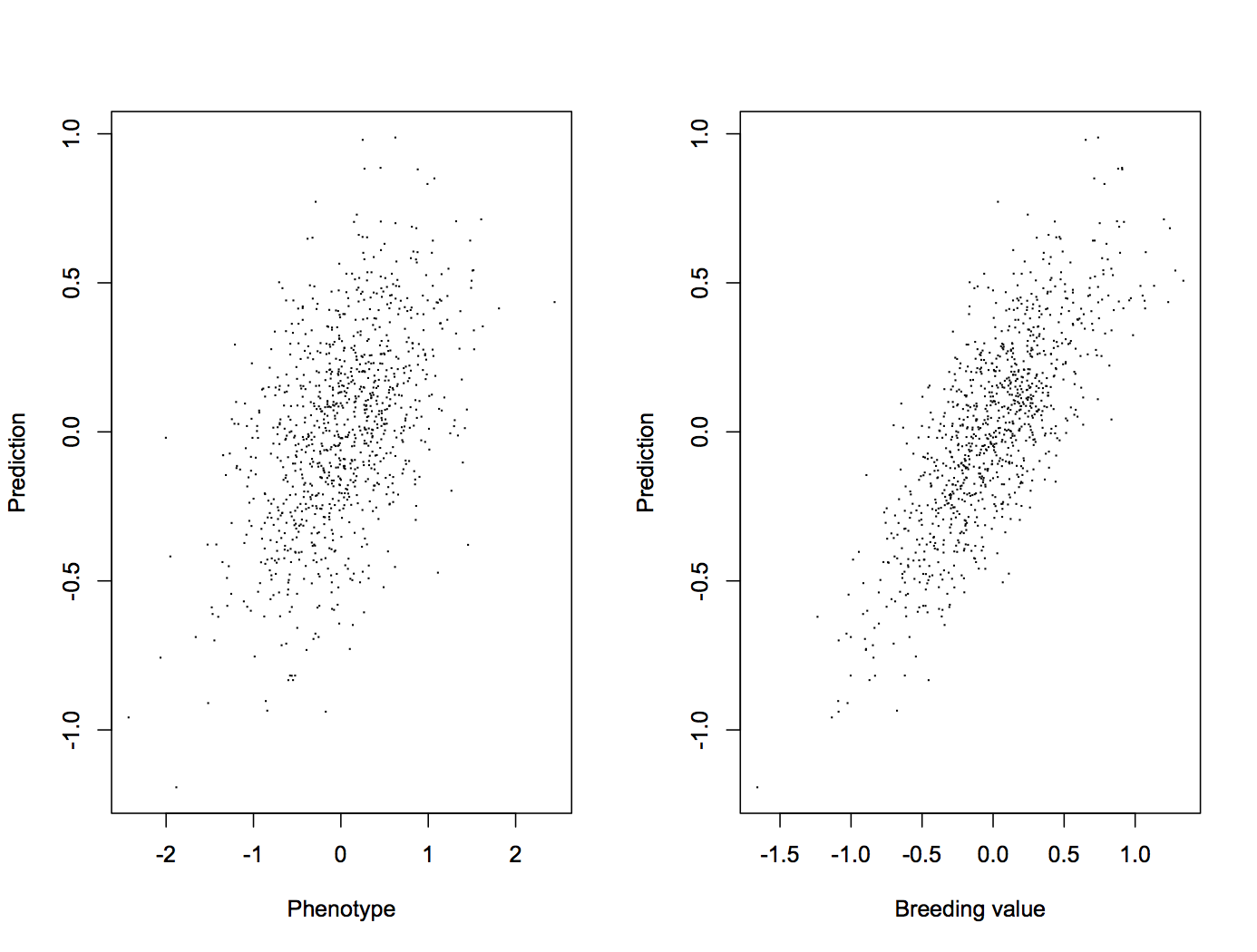
Does it work? Yes, in the sense that it provides genomic estimates for animals that otherwise wouldn’t have any, and that it beats parent average estimates.

Accuracy of GPTA was higher than that of [parent average] for crossbred cows using truncated data from 2012 to predict later phenotypes in 2016 for all traits except productive life. Separate regressions for the 3 BBR categories of crossbreds suggest that the methods perform equally well at 50% BBR, 75% BBR, and 90% BBR.

They mention in passing comparing these estimates to estimates from a common set of marker effects for all breeds, but there is no detail about that model or how it compared in accuracy.

The discussion starts with this sentence:

More breeders now genotype their whole herds and may expect evaluations for all genotyped animals in the future.

That sounds like a reasonable expectation, doesn’t it? Before what they could do with crossbred genotypes was to throw it away. There are lots of other things that might be possible with crossbred evaluation in the future (pulling in crossbred data into the evaluation itself, accounting for ancestry in different parts of the genome, estimating breed-of-origin of alleles, looking at dominance etc etc).

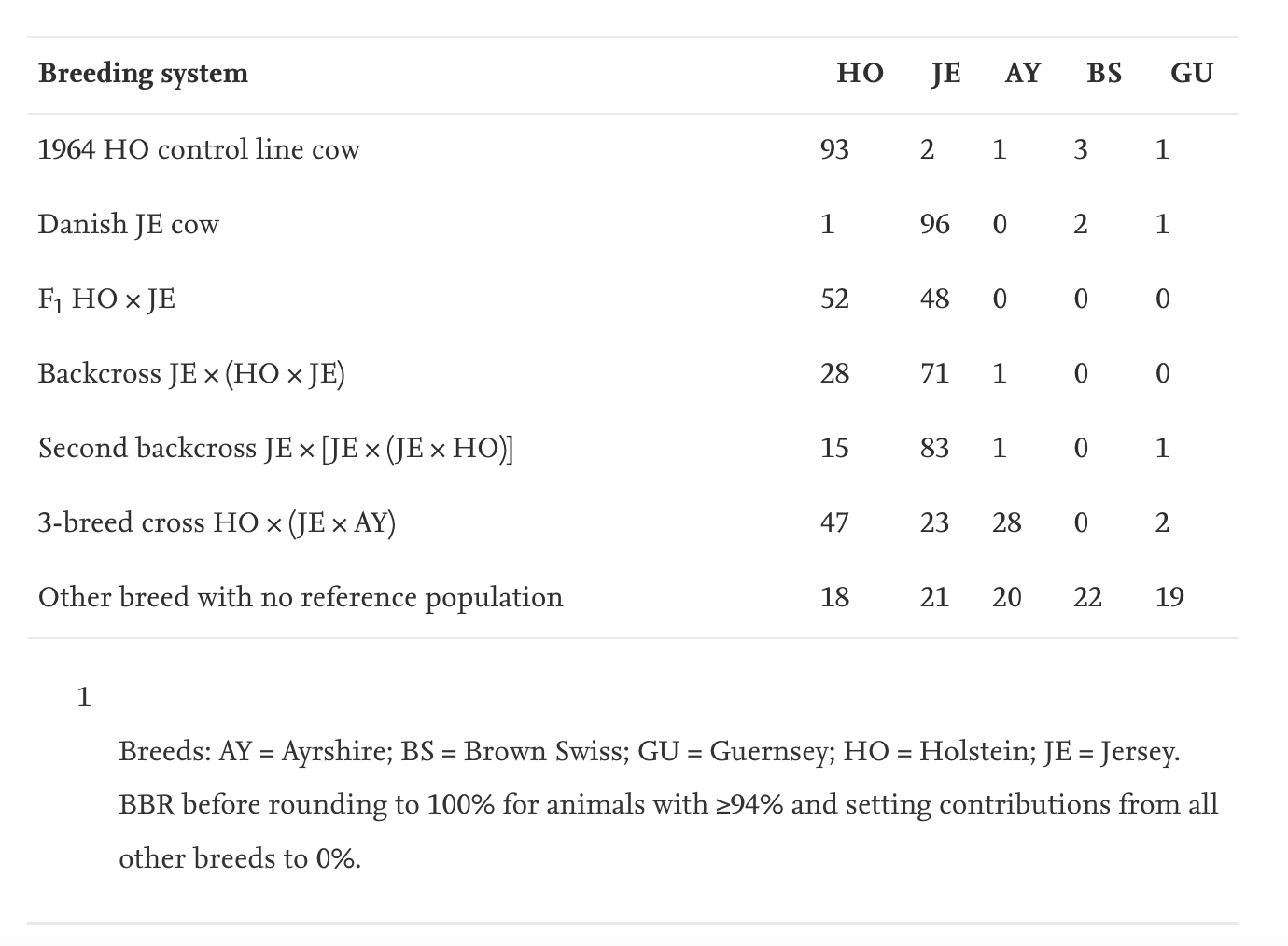
My favourite result in the paper is Table 8, which shows:

Example BBR for animals from different breeding systems are shown in Table 8. The HO cow from a 1964 control line had 1960s genetics from a University of Minnesota experimental selection project and a relatively low relationship to the current HO population because of changes in breed allele frequencies over the past half-century. The Danish JE cow has alleles that differ somewhat from the North American JE population. Other examples in the table show various breed crosses, and the example for an animal from a breed with no reference population shows that genetic contributions from some other breed may be evenly distributed among the included breeds so that BBR percentages sum to 100. These examples illustrate that GBC can be very effective at detecting significant percentages of DNA contributed by another breed.

Literature

VanRaden, P. M., et al. ”Genomic predictions for crossbred dairy cattle.” Journal of Dairy Science 103.2 (2020): 1620-1631.

‘Approaches to genetics for livestock research’ at IASH, University of Edinburgh

A couple of weeks ago, I was at a symposium on the history of genetics in animal breeding at the Institute of Advanced Studies in the Humanities, organized by Cheryl Lancaster. There were talks by two geneticists and two historians, and ample time for discussion.

First geneticists:

Gregor Gorjanc presented the very essence of quantitative genetics: the pedigree-based model. He illustrated this with graphs (in the sense of edges and vertices) and by predicting his own breeding value for height from trait values, and from his personal genomics results.

Then, yours truly gave this talk: ‘Genomics in animal breeding from the perspectives of matrices and molecules’. Here are the slides (only slightly mangled by Slideshare). This is the talk I was preparing for when I collected the quotes I posted a couple of weeks ago.

I talked about how there are two perspectives on genomics: you can think of genomes either as large matrices of ancestry indicators (statistical perspective) or as long strings of bases (sequence perspective). Both are useful, and give animal breeders and breeding researchers different tools (genomic selection, reference genomes). I also talked about potential future breeding strategies that use causative variants, and how they’re not about stopping breeding and designing the perfect animal in a lab, but about supplementing genomic selection in different ways.

Then, historians:

Cheryl Lancaster told the story of how ABGRO, the Animal Breeding and Genetics Research Organisation in Edinburgh, lost its G. The organisation was split up in the 1950s, separating fundamental genetics research and animal breeding. She said that she had expected this split to be do to scientific, methodological or conceptual differences, but instead found when going through the archives, that it all was due to personal conflicts. She also got into how the ABGRO researchers justified their work, framing it as ”fundamental research”, and aspired to do long term research projects.

Jim Lowe talked about the pig genome sequencing and mapping efforts, how it was different from the human genome project in organisation, and how it used comparisons to the human genome a lot. Here he’s showing a photo of Alan Archibald using the gEVAL genome browser to quality-check the pig genome. He also argued that the infrastructural outcomes of a project like the human genome project, such as making it possible for pig genome scientists to use the human genome for comparisons, are more important and less predictable than usually assumed.

The discussion included comments by some of the people who were there (Chris Haley, Bill Hill), discussion about the breed concept, and what scientists can learn from history.

What is a breed? Is it a genetical thing, defined by grouping individuals based on their relatedness, a historical thing, based on what people think a certain kind of animal is supposed to look like, or a marketing tool, naming animals that come from a certain system? It is probably a bit of everything. (I talked with Jim Lowe during lunch; he had noticed how I referred to Griffith & Stotz for gene concepts, but omitted the ”post-genomic” gene concept they actually favour. This is because I didn’t find it useful for understanding how animal breeding researchers think. It is striking how comfortable biologists are with using fuzzy concepts that can’t be defined in a way that cover all corner cases, because biology doesn’t work that way. If the nominal gene concept is broken by trans-splicing, practicing genomicists will probably think of that more as a practical issue with designing gene databases than a something that invalidates talking about genes in principle.)

What would researchers like to learn from history? Probably how to succeed with large research endeavors and how to get funding for them. Can one learn that from history? Maybe not, but there might be lessons about thinking of research as ”basic”, ”fundamental”, ”applied” etc, and about what the long term effects of research might be.

What single step does with relationship

We had a journal club about the single step GBLUP method for genomic evaluation a few weeks ago. In this post, we’ll make a few graphs of how the single step method models relatedness between individuals.

Imagine you want to use genomic selection in a breeding program that already has a bunch of historical pedigree and trait information. You could use some so-called multistep evaluation that uses one model for the classical pedigree + trait quantitative genetics and one model for the genotype + trait genomic evaluation, and then mix the predictions from them together. Or you could use the single-step method, which combines pedigree, genotypes and traits into one model. It does this by combining the relationship estimates from pedigree and genotypes. That matrix can then go into your mixed model.

We’ll illustrate this with a tiny simulated population: five generations of 100 individuals per generation, where ten random pairings produce the next generation, with families of ten individuals. (The R code is on Github and uses AlphaSimR for simulation and AGHmatrix for matrices). Here is a heatmap of the pedigree-based additive relationship matrix for the population:

What do we see? In the lower left corner are the founders, and not knowing anything about their heritage, the matrix has them down as unrelated. The squares of high relatedness along the diagonal are the families in each generation. As we go upwards and to the right, relationship is building up.

Now, imagine the last generation of the population also has been genotyped with a SNP chip. Here is a heatmap of their genomic relationship matrix:

Genomic relationship is more detailed. We can still discern the ten families within the last generation, but no longer are all the siblings equally related to each other and to their ancestors. The genotyping helps track segregation within families, pointing out to us when relatives are more or less related than the average that we get from the pedigree.

Enter the single-step relationship matrix. The idea is to put in the genomic relationships for the genotyped individuals into the big pedigree-based relationship matrix, and then adjust the rest of the matrix to propagate that extra information we now have from the genotyped individuals to their ungenotyped relatives. Here is the resulting heatmap:

You can find the matrix equations in Legarra, Aguilar & Misztal (2009). The matrix, called H, is broken down into four partitions called H11, H12, H21, and H22. H22 is the part that pertains to the genotyped animals, and it’s equal to the genomic relationship matrix G (after some rescaling). The others are transformations of G and the corresponding parts of the additive relationship matrix, spreading G onto A.

To show what is going on, here is the difference between the additive relationship matrix and the single-step relationship matrix, with lines delineating the genotyped animals and breaking the matrix into the four partitions:

What do we see? In the top right corner, we have a lot of difference, where the genomic relationship matrix has been plugged in. Then, fading as we go from top to bottom and from right to left, we see the influence of the genomic relationship on relatives, diminishing the further we get from the genotyped individuals.

Literature

Legarra, Andres, I. Aguilar, and I. Misztal. ”A relationship matrix including full pedigree and genomic information.” Journal of dairy science 92.9 (2009): 4656-4663.

Excerpts about genomics in animal breeding

Here are some good quotes I’ve come across while working on something.

Artificial selection on the phenotypes of domesticated species has been practiced consciously or unconsciously for millennia, with dramatic results. Recently, advances in molecular genetic engineering have promised to revolutionize agricultural practices. There are, however, several reasons why molecular genetics can never replace traditional methods of agricultural improvement, but instead they should be integrated to obtain the maximum improvement in economic value of domesticated populations.

Lande R & Thompson R (1990) Efficiency of marker-assisted selection in the improvement of quantitative traits. Genetics.

Smith and Smith suggested that the way to proceed is to map QTL to low resolution using standard mapping methods and then to increase the resolution of the map in these regions in order to locate more closely linked markers. In fact, future developments should make this approach unnecessary and make possible high resolution maps of the whole genome, even, perhaps, to the level of the DNA sequence. In addition to easing the application of selection on loci with appreciable individual effects, we argue further that the level of genomic information available will have an impact on infinitesimal models. Relationship information derived from marker information will replace the standard relationship matrix; thus, the average relationship coefficients that this represents will be replaced by actual relationships. Ultimately, we can envisage that current models combining few selected QTL with selection on polygenic or infinitesimal effects will be replaced with a unified model in which different regions of the genome are given weights appropriate to the variance they explain.

Haley C & Visscher P. (1998) Strategies to utilize marker–quantitative trait loci associations. Journal of Dairy Science.

Instead, since the late 1990s, DNA marker genotypes were included into the conventional BLUP analyses following Fernando and Grossman (1989): add the marker genotype (0, 1, or 2, for an animal) as a fixed effect to the statistical model for a trait, obtain the BLUP solutions for the additive polygenic effect as before, and also obtain the properly adjusted BLUE solution for the marker’s allele substitution effect; multiply this BLUE by 0, 1, or 2 (specic for the animal) and add the result to the animal’s BLUP to obtain its marker-enhanced EBV. A logical next step was to treat the marker genotypes as semi-random effects, making use of several different shrinkage strategies all based on the marker heritability (e.g., Tsuruta et al., 2001); by 2007, breeding value estimation packages such as PEST (Neumaier and Groeneveld, 1998) supported this strategy as part of their internal calculations. At that time, a typical genetic evaluation run for a production trait would involve up to 30 markers.

Knol EF, Nielsen B, Knap PW. (2016) Genomic selection in commercial pig breeding. Animal Frontiers.

Although it has not caught the media and public imagination as much as transgenics and cloning, genomics will, I believe, have just as great a long-term impact. Because of the availability of information from genetically well-researched species (humans and mice), genomics in farm animals has been established in an atypical way. We can now see it as progressing in four phases: (i) making a broad sweep map (~20 cM) with both highly informative (microsatellite) and evolutionary conserved (gene) markers; (ii) using the informative markers to identify regions of chromosomes containing quantitative trait loci (QTL) controlling commercially important traits–this requires complex pedigrees or crosses between phenotypically anc genetically divergent strains; (iii) progressing from the informative markers into the QTL and identifying trait genes(s) themselves either by complex pedigrees or back-crossing experiments, and/or using the conserved markers to identify candidate genes from their position in the gene-rich species; (iv) functional analysis of the trait genes to link the genome through physiology to the trait–the ‘phenotype gap’.

Bulfield G. (2000) Biotechnology: advances and impact. Journal of the Science of Food and Agriculture.

I believe animal breeding in the post-genomic era will be dramatically different to what it is today. There will be massive research effort to discover the function of genes including the effect of DNA polymorphisms on phenotype. Breeding programmes will utilize a large number of DNA-based tests for specific genes combined with new reproductive techniques and transgenes to increase the rate of genetic improvement and to produce for, or allocate animals to, the product line to which they are best suited. However, this stage will not be reached for some years by which time many of the early investors will have given up, disappointed with the early benefits.

Goddard M. (2003). Animal breeding in the (post-) genomic era. Animal Science.

Genetics is a quantitative subject. It deals with ratios, with measurements, and with the geometrical relationships of chromosomes. Unlike most sciences that are based largely on mathematical techniques, it makes use of its own system of units. Physics, chemistry, astronomy, and physiology all deal with atoms, molecules, electrons, centimeters, seconds, grams–their measuring systems are all reducible to these common units. Genetics has none of these as a recognizable component in its fundamental units, yet it is a mathematically formulated subject that is logically complete and self-contained.

Sturtevant AH & Beadle GW. (1939) An introduction to genetics. W.B. Saunders company, Philadelphia & London.

We begin by asking why genes on nonhomologous chromosomes assort independently. The simple cytological story rehearsed above answers the questions. That story generates further questions. For example, we might ask why nonhomologous chromosomes are distributed independently at meiosis. To answer this question we could describe the formation of the spindle and the migration of chromosomes to the poles of the spindle just before meiotic division. Once again, the narrative would generate yet further questions. Why do the chromosomes ”condense” at prophase? How is the spindle formed? Perhaps in answering these questions we would begin to introduce the chemical details of the process. Yet simply plugging a molecular account into the narratives offered at the previous stages would decrease the explanatory power of those narratives.

Kitcher, P. (1984) 1953 and all that. A tale of two sciences. Philosophical Review.

And, of course, this great quote by Jay Lush.

Summer of data science 1: Genomic prediction machines #SoDS17

Genetics is a data science, right?

One of my Summer of data science learning points was to play with out of the box prediction tools. So let’s try out a few genomic prediction methods. The code is on GitHub, and the simulated data are on Figshare.

Genomic selection is the happy melding of quantitative and molecular genetics. It means using genetic markers en masse to predict traits and and make breeding decisions. It can give you better accuracy in choosing the right plants or animals to pair, and it can allow you to take shortcuts by DNA testing individuals instead of having to test them or their offspring for the trait. There are a bunch of statistical models that can be used for genomic prediction. Now, the choice of prediction algorithm is probably not the most important part of genomic selection, but bear with me.

First, we need some data. For this example, I used AlphaSim (Faux & al 2016), and the AlphaSim graphical user interface, to simulate a toy breeding population. We simulate 10 chromosomes á 100 cM, with 100 additively acting causal variants and 2000 genetic markers per chromosome. The initial genotypes come from neutral simulations. We run one generation of random mating, then three generations of selection on trait values. Each generation has 1000 individuals, with 25 males and 500 females breeding.

So we’re talking a small-ish population with a lot of relatedness and reproductive skew on the male side. We will use the two first two generations of selection (2000 individuals) to train, and try to predict the breeding values of the fourth generation (1000 individuals). Let’s use two of the typical mixed models used for genomic selection, and two tree methods.

We start by splitting the dataset and centring the genotypes by subtracting the mean of each column. Centring will not change predictions, but it may help with fitting the models (Strandén & Christensen 2011).

Let’s begin with the workhorse of genomic prediction: the linear mixed model where all marker coefficients are drawn from a normal distribution. This works out to be the same as GBLUP, the GCTA model, GREML, … a beloved child has many names. We can fit it with the R package BGLR. If we predict values for the held-out testing generation and compare with the real (simulated) values, it looks like this. The first panel shows a comparison with phenotypes, and the second with breeding values.

This gives us correlations of 0.49 between prediction and phenotype, and 0.77 between prediction and breeding value.

This is a plot of the Markov chain Monte Carlo we use to sample from the model. If a chain behaves well, it is supposed to have converged on the target distribution, and there is supposed to be low autocorrelation. Here is a trace plot of four chains for the marker variance (with the coda package). We try to be responsible Bayesian citizens and run the analysis multiple times, and with four chains we get very similar results from each of them, and a potential scale reduction factor of 1.01 (it should be close to 1 when it works). But the autocorrelation is high, so the chains do not explore the posterior distribution very efficiently.

BGLR can also fit a few of the ”Bayesian alphabet” variants of the mixed model. They put different priors on the distribution of marker coefficients allow for large effect variants. BayesB uses a mixture prior, where a lot of effects are assumed to be zero (Meuwissen, Hayes & Goddard 2001). The way we simulated the dataset is actually close to the BayesB model: a lot of variants have no effect. However, mixture models like BayesB are notoriously difficult to fit — and in this case, it clearly doesn’t work that well. The plots below show chains for two BayesB parameters, with potential scale reduction factors of 1.4 and 1.5. So, even if the model gives us the same accuracy as ridge regression (0.77), we can’t know if this reflects what BayesB could do.

On to the trees! Let’s try Random forest and Bayesian additive regression trees (BART). Regression trees make models as bifurcating trees. Something like the regression variant of: ”If the animal has a beak, check if it has a venomous spur. If it does, say that it’s a platypus. If it doesn’t, check whether it quacks like a duck …” The random forest makes a lot of trees on random subsets of the data, and combines the inferences from them. BART makes a sum of trees. Both a random forest (randomForest package) and a BART model on this dataset (fit with bartMachine package), gives a lower accuracy — 0.66 for random forest and 0.72 for BART. This is not so unexpected, because the strength of tree models seems to lie in capturing non-additive effects. And this dataset, by construction, has purely additive inheritance. Both BART and random forest have hyperparameters that one needs to set. I used package defaults for random forest, values that worked well for Waldmann (2016), but one probably should choose them by cross validation.

Finally, we can use classical quantitative genetics to estimate breeding values from the pedigree and relatives’ trait values. Fitting the so called animal model in two ways (pedigree package and MCMCglmm) give accuracies of 0.59 and 0.60.

So, in summary, we recover the common wisdom that the linear mixed model does the job well. It was more accurate than just pedigree, and a bit better than BART. Of course, the point of this post is not to make a fair comparison of methods. Also, the real magic of genomic selection, presumably, happens on every step of the way. How do you get to that neat individual-by-marker matrix in the first place, how do you deal with missing data and data from different sources, what and when do you measure, what do you do with the predictions … But you knew that already.