Journal club of one: ”Genome-wide enhancer maps link risk variants to disease genes”

(Here is a a paper from a recent journal club.)

Nasser et al. (2021) present a way to prioritise potential noncoding causative variants. This is part of solving the fine mapping problem, i.e. how to find the underlying causative variants from genetic mapping studies. They do it by connecting regulatory elements to genes and overlapping those regulatory elements with variants from statistical fine-mapping. Intuitively, it might not seem like connecting regulatory elements to genes should be that hard, but it is a tricky problem. Enhancers — because that is the regulatory element most of this is about; silencers and insulators get less attention — do not carry any sequence that tells us what gene they will act on. Instead, this needs to be measured or predicted somehow. These authors go the measurement route, combining chromatin sequencing with chromosome conformation capture.

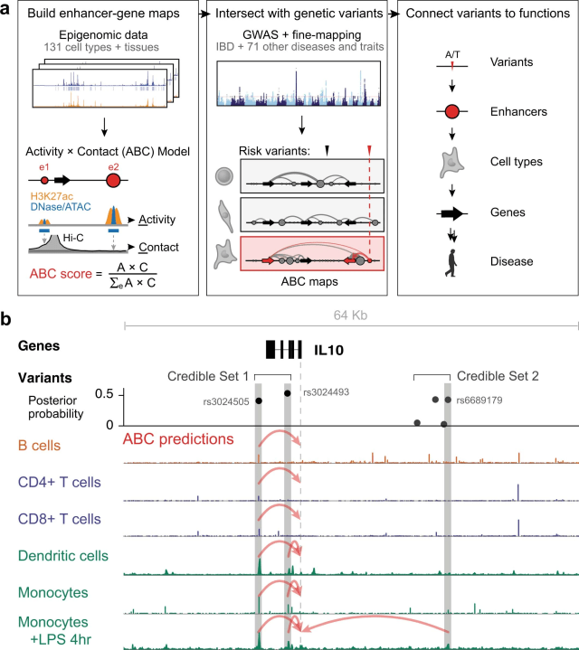
This figure from the supplementary materials show what the method is about:

Additional figure 1 from Nasser et al. (2021) showing an overview of the workflow and an example of two sets of candidate variants derived from-fine mapping, each with variants that overlap enhancers connected to IL10.

They use chromatin sequence data (such as ATAC-seq, histone ChIP-seq or DNAse-seq) in combination with HiC chromosome conformation capture data to identify enhancers and connect them to genes (this was developed earlier in Fulco et al. 2019). The ”activity-by-contact model” means to multiply the contact frequency (from HiC) between promoter and enhancer with the enhancer activity (read counts from chromatin sequencing), standardised by the total contact–activity product with all elements within a window. Fulco et al. (2019) previously found that this conceptually simple model did well at connecting enhancers to genes (as evaluated with a CRISPR inhibition assay called CRISPRi-FlowFISH, which we’re not going into now, but it’s pretty ingenious).

In order to use this for fine-mapping, they calculated activity-by-contact maps for every gene combined with every open chromatin element within 5 Mbp for 131 samples from ENCODE and other sources. The HiC data were averaged of contacts in ten cell types, transformed to be follow a power-law distribution. That is, they did not do the HiC analysis per cell type, but use the same average HiC contact matrix combined with chromatin data from different cell types. Thus, the specificity comes from the promoters and enhancers that are called as active in each sample — I assume this is because the HiC data comes from a different (and smaller) set of cell types than the chromatin sequencing. Element–gene pairs that reached above a threshold were considered connected, for a total of about six million connections, involving 23,000 genes and 270,000 enhancers. On average, a gene had 2.8 enhancers and an enhancer connected to 2.7 genes.

They picked putative causative variants by overlapping the variant sets with these activity-by-contact maps and selecting the highest scoring enhancer gene pair.They used fine-mapping results from multiple previous studies. These variants were estimated with different methods, but they are all some flavour of fine-mapping by variable selection. Statistical fine mapping estimate sets of variants, called credible sets, that have high posterior probability of being the causative variant. They included only completely noncoding credible sets, i.e. those that did not include a coding sequence or splice variant. They applied this to 72 traits in humans, generating predictions for ~ 5000 noncoding credible sets of variants.

Did it work?

Variants for fine-mapping were enriched in connected enhancers more than in open chromatin in general, in cell types that are relevant to the traits. In particular, inflammatory bowel disease variants were enriched in enhancers in 65 samples, including immune cell types and gut cells. The strongest enrichment was in activated dendritic cells.

They used a set of genes previously known to be involved in inflammatory bowel disease, assuming that they were the true causative genes for their respective noncoding credible sets, and then compared their activity-by-contact based prioritisation of the causative gene to simply picking the closest gene. Picking the closest gene was right in 30 out of 37 sets. Picking the gene with the highest activity-by-contact score was right in 17 cases out of 18 sets that overlapped an activity-by-contact enhancer. Thus, this method had higher precision but worse recall. They also tested a number of eQTL-based, enrichment and enhancer–gene mapping methods, that did worse.

What it tells us about causative variants

Most of the putative causative variants, picked based on maximising activity-by-contact, were close to the proposed gene (median 13 kbp) and most involved the closest gene (77%). They were often found their putative causative variants to be located in enhancers that were only active in a few cell- or tissue types (median 4), compared to the promoters of the target genes, that were active in a broader set (median 120). For example, in inflammatory bowel disease, there were several examples where the putatively causal enhancer was only active in a particular immune cell or a stimulated state of an immune cell.

My thoughts

What I like about this model is that it is so different to many of the integrative and machine learning methods we see in genomics. It uses two kinds of data, and relatively simple computations. There is no machine learning. There is no sequence evolution or conservation analysis. Instead, measure two relevant quantities, standardise and preprocess them a bit, and then multiply them together.

If the success of the activity-by-contact model for prioritising causal enhancers generalises beyond the 18 causative genes investigated in the original paper, this is an argument for simple biology-based heuristics over machine learning models. It also suggest that, in the absence of contact data, one might do well by prioritising variant in enhancers that are highly active in relevant cell types, and picking the closest gene as the proposed causative gene.

However, the dataset needs to cover the relevant cell types, and possibly cells that are in the relevant stimulated states, meaning that it provides a motivation for rich conditional atlas-style datasets of chromatin and chromosome conformation.

I am, personally, a little bit sad that expression QTL methods seem to doing poorly. On the other hand, it makes some sense that eQTL might not have the genomic resolution to connect enhancers to genes.

Finally, if the relatively simple activity-by-contact model or the ridiculously simple method of ”picking the closest gene” beats machine learning models using the same data types and more, it suggests that the machine learning methods might not be solving theright problem. After all, they are not trained directly to prioritise variants for complex traits — because there are too few known causative variants for complex traits.

Literature

Fulco, C. P., Nasser, J., Jones, T. R., Munson, G., Bergman, D. T., Subramanian, V., … & Engreitz, J. M. (2019). Activity-by-contact model of enhancer–promoter regulation from thousands of CRISPR perturbations. Nature genetics.

Nasser, J., Bergman, D. T., Fulco, C. P., Guckelberger, P., Doughty, B. R., Patwardhan, T. A., … & Engreitz, J. M. (2021). Genome-wide enhancer maps link risk variants to disease genes. Nature.
Journal club of one: ”Chromosome-level and haplotype-resolved genome assembly enabled by high-throughput single-cell sequencing of gamete genomes”

Genome assembly researchers are still figuring out new wild ways of combining different kinds of data. For example, ”trio binning” took what used to be a problem, — the genetic difference between the two genome copies that a diploid individual carries — and turned it into a feature: if you assemble a hybrid individual with genetically distant parents, you can separate the two copies and get two genomes in one. (I said that admixture was the future of every part of genetics, didn’t I?) This paper (Campoy et al. 2020) describes ”gamete binning” which uses sequencing of gametes perform a similar trick.

Expressed another way, gamete binning means building an individual-specific genetic map and then using it to order and phase the pieces of the assembly. This means two sequence datasets from the same individual — one single cell short read dataset from gametes (10X linked reads) and one long read dataset from the parent (PacBio) — and creatively re-using them in different ways.

This is what they do:

1. Assemble the long reads into a preliminary assembly, which will be a mosaic of the two genome copies (barring gross differences, ”haplotigs”, that can to some extent be removed).

2. Align the single cell short reads to the preliminary assembly and call SNPs. (They also did some tricks to deal with regions without SNPs, separating those that were not variable between genomes and those that were deleted in one genome.) Because the gametes are haploid, they get the phase of the parent’s genotype.

3. Align the long reads again. Now, based on the phased genotype, the long reads can be assigned to the genome copy they belong to. So they can partition the reads into one bin per genome copy and chromosome.

4. Assemble those bins separately. They now get one assembly for each homologous chromosome.

They apply it to an apricot tree, which has a 250 Mbp genome. When they sequence the parents of the tree, it seems to separate the genomes well. The two genome copies have quite a bit of structural variation:

Despite high levels of synteny, the two assemblies revealed large-scale rearrangements (23 inversions, 1,132 translocation/transpositions and 2,477 distal duplications) between the haplotypes making up more than 15% of the assembled sequence (38.3 and 46.2 Mb in each of assemblies; Supplementary Table 1). /…/ Mirroring the huge differences in the sequences, we found the vast amount of 942 and 865 expressed, haplotype-specific genes in each of the haplotypes (Methods; Supplementary Tables 2-3).

They can then go back to the single cell data and look at the recombination landscape and at chromosomal arrangements during meiosis.

This is pretty elegant. I wonder how dependent it is on the level of variation within the individual, and how it compares in cost and finickiness to other assembly strategies.

Literature

Campoy, José A., et al. ”Chromosome-level and haplotype-resolved genome assembly enabled by high-throughput single-cell sequencing of gamete genomes.” BioRxiv (2020).

Journal club of one: ”Versatile simulations of admixture and accurate local ancestry inference with mixnmatch and ancestryinfer”

Admixture is the future of every sub-field of genetics, just in case you didn’t know. Both in the wild and domestic animals, populations or even species sometimes cross. This causes different patterns of relatedness than in well-mixed populations. Often we want to estimate ”local ancestry”, that is: what source population a piece of chromosome in an individual originates from. It is one of those genetics problems that is made harder by the absence of any way to observe it directly.

This recent paper (Schumer et al 2020; preprint version, which I read, here) presents a method for simulating admixed sequence data, and a method for inferring local ancestry from it. It does something I like, namely to pair analysis with fake-data simulation to check methods.

The simulation method is a built from four different simulators:

1. macs (Chen, Majoram & Wall 2009), which creates polymorphism data under neutral evolution from a given population history. They use macs to generate starting chromosomes from two ancestral populations.

2. Seq-Gen (Rambaut & Grassly 1997). Chromosomes from macs are strings of 0s and 1s representing the state at biallelic markers. If you want DNA-level realism, with base composition, nucleotide substitution models and so on, you need something else. I don’t really follow how they do this. You can tell from the source code that they use the local trees that macs spits out, which Seq-Gen can then simulate nucleotides from. As they put it, the resulting sequence ”lacks other complexities of real genome sequences such as repetitive elements and local variation in base composition”, but it is a step up from ”0000110100”.

3. SELAM (Corbett-Detig & Jones 2016), which simulates admixture between populations with population history and possibly selection. Here, SELAM‘s role is to simulate the actual recombination and interbreeding to create the patterns of local ancestry, that they will then fill with the sequences they generated before.

4. wgsim, which simulates short reads from a sequence. At this point, mixnmatch has turned a set of population genetic parameters into fasta files. That is pretty cool.

On the one hand, building on tried and true tools seems to be the right thing to do, less wheel-reinventing. It’s great that the phylogenetic simulator Seq-Gen from 1997 can be used in a paper published in 2020. On the other hand, looking at the dependencies for running mixnmatch made me a little pale: seven different bioinformatics or population genetics softwares (not including the dependencies you need to compile them), R, Perl and Python plus Biopython. Computational genetics is an adventure of software installation.

They use the simulator to test the performance of a hidden Markov model for inferring local ancestry (Corbett-Detig & Nielsen 2017) with different population histories and settings, and then apply it to swordtail fish data. In particular, one needs to set thresholds for picking ”ancestry informative” (i.e. sufficiently differentiated) markers between the ancestral populations, and that depends on population history and diversity.

In passing, they use the estimate the swordtail recombination landscape:

We used the locations of observed ancestry transitions in 139 F2 hybrids that we generated between X. birchmanni and X. malinche … to estimate the recombination rate in 5 Mb windows. … We compared inferred recombination rates in this F2 map to a linkage disequilibrium based recombination map for X. birchmanni that we had previously generated (Schumer et al., 2018). As expected, we observed a strong correlation in estimated recombination rate between the linkage disequilibrium based and crossover maps (R=0.82, Figure 4, Supporting Information 8). Simulations suggest that the observed correlation is consistent with the two recombination maps being indistinguishable, given the low resolution of the F2 map (Supporting Information 8).

Journal club of one: ”Eliciting priors and relaxing the single causal variant assumption in colocalisation analyses”

This paper (Wallace 2020) is about improvements to the colocalisation method for genome-wide association studies called coloc. If you have an association to trait 1 in a region, and another association with trait 2, coloc investigates whether they are caused by the same variant or not. I’ve never used coloc, but I’m interested because setting reasonable priors is related to getting reasonable parameters for genetic architecture.

The paper also looks at how coloc is used in the literature (with default settings, unsurprisingly), and extends coloc to relax the assumption of only one causal variant per region. In that way, it’s a solid example of thoughtfully updating a popular method.

(A note about style: This isn’t the clearest paper, for a few reasons. The structure of the introduction is indirect, talking a lot about Mendelian randomisation before concluding that coloc isn’t Mendelian randomisation. The paper also uses numbered hypotheses H1-H4 instead of spelling out what they mean … If you feel a little stupid reading it, it’s not just you.)

coloc is what we old QTL mappers call a pleiotropy versus linkage test. It tries to distinguish five scenarios: no association, trait 1 only, trait 2 only, both traits with linked variants, both traits with the same variant.

This paper deals with the priors: What is the prior probability of a causal association to trait 1 only p_1, trait 2 only p_2, or both traits p_{12} , and are the defaults good?

They reparametrise the priors so that it becomes possible to get some estimates from the literature. They work with the probability that a SNP is causally associated with each trait (which means adding the probabilities of association q_1 = p_1 + p_{12} ) … This means that you can look at single trait association data, and get an idea of the number of marginal associations, possibly dependent on allele frequency. The estimates from a gene expression dataset and a genome-wide association catalog work out to a prior around 10 ^ {-4} , which is the coloc default. So far so good.

How about p_{12} ?

If traits were independent, you could just multiply q_1 and q_2. But not all of the genome is functional. If you could straightforwardly define a functional proportion, you could just divide by it.

You could also look at the genetic correlation between traits. It makes sense that the overall genetic relationship between two traits should inform the prior that you see overlap at this particular locus. This gives a lower limit for p_{12} . Unfortunately, this still leaves us dependent on what kinds of traits we’re analysing. Perhaps, it’s not so surprising that there isn’t one prior that universally works for all kinds of pairs of trait:

Attempts to colocalise disease and eQTL signals have ranged from underwhelming to positive. One key difference between outcomes is the disease-specific relevance of the cell types considered, which is consistent with variable chromatin state enrichment in different GWAS according to cell type. For example, studies considering the overlap of open chromatin and GWAS signals have convincingly shown that tissue relevance varies by up to 10 fold, with pancreatic islets of greatest relevance for traits like insulin sensitivity and immune cells for immune-mediated diseases. This suggests that p_{12} should depend explicitly on the specific pair of traits under consideration, including cell type in the case of eQTL or chromatin mark studies. One avenue for future exploration is whether fold change in enrichment of open chromatin/GWAS signal overlap between cell types could be used to modulate p_{12} and select larger values for more a priori relevant tissues.

Literature

Wallace, Chris. ”Eliciting priors and relaxing the single causal variant assumption in colocalisation analyses.” PLoS Genetics 16.4 (2020): e1008720.

Journal club of one: ”Genomic predictions for crossbred dairy cattle”

A lot of dairy cattle is crossbred, but genomic evaluation is often done within breed. What about the crossbred individuals? This paper (VanRaden et al. 2020) describes the US Council on Dairy Cattle Breeding’s crossbred genomic prediction that started 2019.

In short, the method goes like this: They describe each crossbred individual in terms of their ”genomic breed composition”, get predictions for each them based on models from all the breeds separately, and then combine the results in proportion to the genomic breed composition. The paper describes how they estimate the genomic breed composition, and evaluated accuracy by predicting held-out new data from older data.

The genomic breed composition is a delightfully elegant hack: They treat ”how much breed X is this animal” as a series of traits and run a genomic evaluation on them. The training set: individuals from sets of reference breeds with their trait value set to 100% for the breed they belong to and 0% for other breeds. ”Marker effects for GBC [genomic breed composition] were then estimated using the same software as for all other traits.” Neat. After some adjustment, they can be interpreted as breed percentages, called ”base breed representation”.

As they already run genomic evaluations from each breed, they can take these marker effects and then animal’s genotypes, and get one estimate for each breed. Then they combine them, weighting by the base breed representation.

Does it work? Yes, in the sense that it provides genomic estimates for animals that otherwise wouldn’t have any, and that it beats parent average estimates.

Accuracy of GPTA was higher than that of [parent average] for crossbred cows using truncated data from 2012 to predict later phenotypes in 2016 for all traits except productive life. Separate regressions for the 3 BBR categories of crossbreds suggest that the methods perform equally well at 50% BBR, 75% BBR, and 90% BBR.

They mention in passing comparing these estimates to estimates from a common set of marker effects for all breeds, but there is no detail about that model or how it compared in accuracy.

The discussion starts with this sentence:

More breeders now genotype their whole herds and may expect evaluations for all genotyped animals in the future.

That sounds like a reasonable expectation, doesn’t it? Before what they could do with crossbred genotypes was to throw it away. There are lots of other things that might be possible with crossbred evaluation in the future (pulling in crossbred data into the evaluation itself, accounting for ancestry in different parts of the genome, estimating breed-of-origin of alleles, looking at dominance etc etc).

My favourite result in the paper is Table 8, which shows:

Example BBR for animals from different breeding systems are shown in Table 8. The HO cow from a 1964 control line had 1960s genetics from a University of Minnesota experimental selection project and a relatively low relationship to the current HO population because of changes in breed allele frequencies over the past half-century. The Danish JE cow has alleles that differ somewhat from the North American JE population. Other examples in the table show various breed crosses, and the example for an animal from a breed with no reference population shows that genetic contributions from some other breed may be evenly distributed among the included breeds so that BBR percentages sum to 100. These examples illustrate that GBC can be very effective at detecting significant percentages of DNA contributed by another breed.

Literature

VanRaden, P. M., et al. ”Genomic predictions for crossbred dairy cattle.” Journal of Dairy Science 103.2 (2020): 1620-1631.

Journal club of one: ”Evolutionary stalling and a limit on the power of natural selection to improve a cellular module”

This is a relatively recent preprint on how correlations between genetic variants can limit the response to selection, with experimental evolution in bacteria.

Experimental evolution and selection experiments live on the gradient from modelling to observations in the wild. Experimental evolution researchers can design the environments and the genotypes to pose problems for evolution, and then watch in real time as organisms solve them. With sequencing, they can also watch how the genome responds to selection.

In this case, the problem posed is how to improve a particular cellular function (”module”). The researcher started out with engineered Escherichia coli that had one component of their translation machinery manipulated: they started out with only one copy of an elongation factor gene (where E.coli normally has two) that could be either from another species, an reconstructed ancestral form, or the regular E.coli gene as a control.

Then, they sequenced samples from replicate populations over time, and looked for potentially adaptive variants: that is, operationally, variants that had large changes in frequency (>20%) and occurred in genes that had more than one candidate adaptive variant.

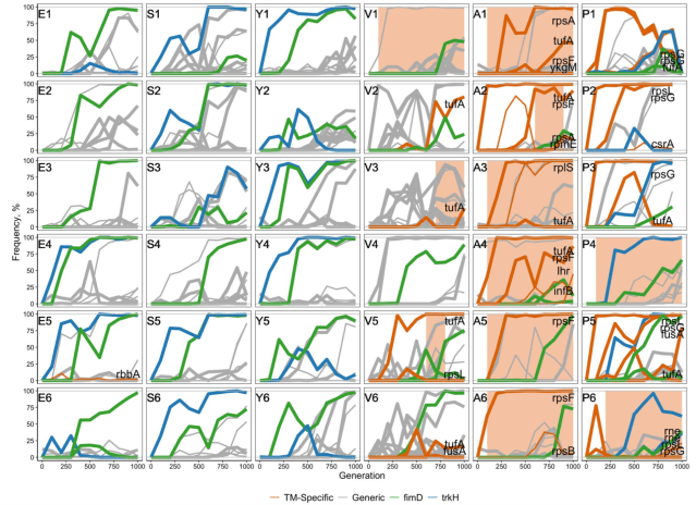
Finally, because they looked at what genes these variants occurred in. Were they related to translation (”TM-specific” as they call it) or not (”generic”). That gave them trajectories of potentially adaptive variants like this. The horizontal axis is time and the vertical frequency of the variant. The letters are populations of different origin, and the numbers replicates thereof. The colour shows the classification of variants. (”fimD” and ”trkH” in the figure are genes in the ”generic” category that are of special interest for other reasons. The orange–brown shading signifies structural variation at the elongation factor gene.)

This figure shows their main observations:

  • V, A and P populations had more adaptive variants in translation genes, and also worse fitness at the start of the experiment. This goes together with improving more during the experiment. If a population has poor translation, a variant in a translation gene might help. If it has decent translation efficiency already, there is less scope for improvement, and adaptive variants in other kinds of genes happen more often.

    We found that populations whose TMs were initially mildly perturbed (incurring ≲ 3% fitness cost) adapted by acquiring mutations that did not directly affect the TM. Populations whose TM had a moderately severe defect (incurring ~19% fitness cost) discovered TM-specific mutations, but clonal interference often prevented their fixation. Populations whose TMs were initially severely perturbed (incurring ~35% fitness cost) rapidly discovered and fixed TM-specific beneficial mutations.

  • Adaptive variants in translation genes tended to increase fast and early during the experiment and often get fixed, suggesting that they have larger effects than. Again, the your translation capability is badly broken, a large-effect variant in a translation gene might help.

    Out of the 14 TM-specific mutations that eventually fixed, 12 (86%) did so in the first selective sweep. As a result, an average TM-specific beneficial mutation reached fixation by generation 300 ± 52, and only one (7%) reached fixation after generation 600 … In contrast, the average fixation time of generic mutations in the V, A and P populations was 600 ± 72 generations, and 9 of them (56%) fixed after the first selective sweep

  • After one adaptive variant in a translation gene, it seems to stop at that.

The question is: when there aren’t further adaptive variants in translation genes, is that because it’s impossible to improve translation any further, or because of interference from other variants? They use the term ”evolutionary stalling”, kind of asexual linked selection. Because variants occur together, selection acts on the net effect of all the variants in an individual. Adaptation in a certain process (in this case translation) might stall, if there are large-effect adaptive variants in other, potentially completely unrelated processes, that swamp the effect on translation.

They argue for three kinds of indirect evidence that the adaptation in translation has stalled in at least some of the populations:

  1. Some of the replicate populations of V didn’t fix adaptive translation variants.
  2. In some populations, there were a second adaptive translation variant, not yet fixed.
  3. There have been adaptive translation mutations in the Long Term Evolution Experiment, which is based on E.coli with unmanipulated translation machinery.

Stalling depends on large-effect variants, but after they have fixed, adaptation might resume. They use the metaphor of natural selection ”shifting focus”. The two non-translation genes singled out in the above figure might be examples of that:

While we did not observe resumption of adaptive evolution in [translation] during the duration of this experiment, we find evidence for a transition from stalling to adaptation in trkH and fimD genes. Mutations in these two genes appear to be beneficial in all our genetic backgrounds (Figure 4). These mutations are among the earliest to arise and fix in E, S and Y populations where the TM does not adapt … In contrast, mutations in trkH and fimD arise in A and P populations much later, typically following fixations of TM-specific mutations … In other words, natural selection in these populations is initially largely focused on improving the TM, while adaptation in trkH and fimD is stalled. After a TM-specific mutation is fixed, the focus of natural selection shifts away from the TM to other modules, including trkH and fimD.

This is all rather indirect, but interesting. Both ”the focus of natural selection shifting” and ”coupling of modules by the emergent neutrality threshold” are inspiring ways to think about the evolution of genetic architecture, and new to me.

Literature

Venkataram, Sandeep, et al. ”Evolutionary Stalling and a Limit on the Power of Natural Selection to Improve a Cellular Module.” bioRxiv (2019): 850644.

Journal club: ”Template plasmid integration in germline genome-edited cattle”

(This time it’s not just a Journal Club of One, because this post is based on a presentation given at the Hickey group journal club.)

The backstory goes like this: Polled cattle lack horns, and it would be safer and more convenient if more cattle were born polled. Unfortunately, not all breeds have a lot of polled cattle, and that means that breeding hornless cattle is difficult. Gene editing could help (see Bastiaansen et al. (2018) for a model).

In 2013, Tan et al. reported taking cells from horned cattle and editing them to carry the polled allele. In 2016, Carlson et al. cloned bulls based on a couple of these cell lines. The plan was to use the bulls, now grown, to breed polled cattle in Brazil (Molteni 2019). But a few weeks ago, FDA scientists (Norris et al 2019) posted a preprint that found inadvertent plasmid insertion in the bulls, using the public sequence data from 2016. Recombinetics, the company making the edited bulls, conceded that they’d missed the insertion.

”We weren’t looking for plasmid integrations,” says Tad Sonstegard, CEO of Recombinetics’ agriculture subsidiary, Acceligen, which was running the research with a Brazilian consulting partner. ”We should have.”

Oops.

For context: To gene edit a cell, one needs to bring both the editing machinery (proteins in the case of TALENS, the method used here; proteins and RNA in the case of CRISPR) and the template DNA into the cell. The template DNA is the DNA you want to put in instead of the piece that you’re changing. There are different ways to get the components into the cell. In this case, the template was delivered as part of a plasmid, which is a bacterially-derived circular DNA.

The idea is that the editing machinery should find a specific place in the genome (where the variant that causes polledness is located), make a cut in the DNA, and the cell, in its efforts to repair the cut, will incorporate the template. Crucially, it’s supposed to incorporate only the template, and not the rest of the plasmid. But in this case, the plasmid DNA snuck in too, and became part of the edited chromosome. Biological accidents happen.

How did they miss that, and how did the FDA team detect it? Both the 2016 and 2019 paper are short letters where a lot of the action is relegated to the supplementary materials. Here are pertinent excerpts from Carlson & al 2016:

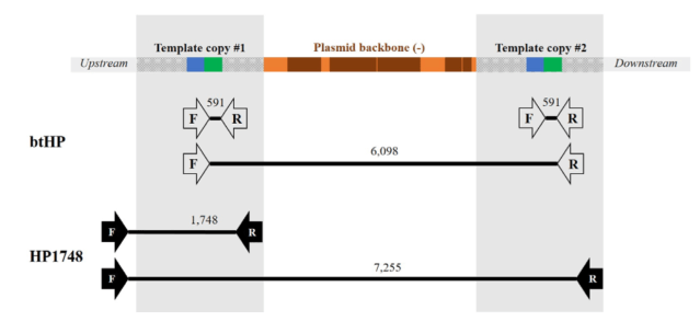
A first PCR assay was performed using (btHP-F1: 5’- GAAGGCGGCACTATCTTGATGGAA; btHP-R2- 5’- GGCAGAGATGTTGGTCTTGGGTGT) … The PCR creates a 591 bp product for Pc compared to the 389 bp product from the horned allele.

Secondly, clones were analyzed by PCR using the flanking F1 and R1 primers (HP1748-F1- 5’- GGGCAAGTTGCTCAGCTGTTTTTG; HP1594_1748-R1- 5’-TCCGCATGGTTTAGCAGGATTCA) … The PCR creates a 1,748 bp product for Pc compared to the 1,546 bp product from the horned allele.

All PCR products were TOPO cloned and sequenced.

Thus, they checked that the animals were homozygotes for the polled allele (called ”Pc”) by amplifying two diagnostic regions and sequenced them to check the edit. This shows that the target DNA is there.

Then, they used whole-genome short read sequencing to check for off-target edits:

Samples were sequenced to an average 20X coverage on the Illumina HiSeq 2500 high output mode with paired end 125 bp reads were compared to the bovine reference sequence (UMD3.1).

Structural variations were called using CLC probabilistic variant detection tools, and those with >7 reads were further considered even though this coverage provides only a 27.5% probability of accurately detecting heterozygosity.

Upon indel calls for the original non-edited cell lines and 2 of the edited animals, we screened for de novo indels in edited animal RCI-001, which are not in the progenitor cell-line, 2120.

We then applied PROGNOS4 with reference bovine genome build UMD3.1 to compute all potential off-targets likely caused by the TALENs pair.

For all matching sequences computed, we extract their corresponding information for comparison with de novo indels of RCI-001 and RCI-002. BEDTools was adopted to find de novo indels within 20 bp distance of predicted potential targets for the edited animal.

Only our intended edit mapped to within 10 bp of any of the identified degenerate targets, revealing that our animals are free of off-target events and further supporting the high specificity of TALENs, particularly for this locus.

That means, they sequenced the animals’ genomes in short fragment, puzzled it together by aligning it to the cow reference genome, and looked for insertions and deletions in regions that look similar enough that they might also be targeted by their TALENs and cut. And because they didn’t find any insertions or deletions close to these potential off-target sites, they concluded that the edits were fine.

The problem is that short read sequencing is notoriously bad at detecting larger insertions and deletions, especially of sequences that are not in the reference genome. In this case, the plasmid is not normally part of a cattle genome, and thus not in the reference genome. That means that short reads deriving from the inserted plasmid sequence would probably not be aligned anywhere, but thrown away in the alignment process. The irony is that with short reads, the bigger something is, the harder it is to detect. If you want to see a plasmid insertion, you have to make special efforts to look for it.

Tan et al. (2013) were aware of the risk of plasmid insertion, though, at least when concerned with the plasmid delivering the TALEN. Here is a quote:

In addition, after finding that one pair of TALENs delivered as mRNA had similar activity as plasmid DNA (SI Appendix, Fig. S2), we chose to deliver TALENs as mRNA to eliminate the possible genomic integration of TALEN expression plasmids. (my emphasis)

As a sidenote, the variant calling method used to look for off-target effects (CLC Probabilistic variant detection) doesn’t even seem that well suited to the task. The manual for the software says:

The size of insertions and deletions that can be found depend on how the reads are mapped: Only indels that are spanned by reads will be detected. This means that the reads have to align both before and after the indel. In order to detect larger insertions and deletions, please use the InDels and Structural Variation tool instead.

The CLC InDels and Structural Variation tool looks at the unaligned (soft-clipped) ends of short sequence reads, which is one way to get at structural variation with short read sequences. However, it might not have worked either; structural variation calling is a hard task, and the tool does not seem to be built for this kind of task.

What did Norris & al (2019) do differently? They took the published sequence data and aligned it to a cattle reference genome with the plasmid sequence added. Then, they loaded the alignment into the trusty Integrative Genomics Viewer and manually looked for reads aligning to the plasmid and reads supporting junctions between plasmid, template DNA and genome. This bespoken analysis is targeted to find plasmid insertions. The FDA authors must have gone ”nope, we don’t buy this” and decided to look for the plasmid.

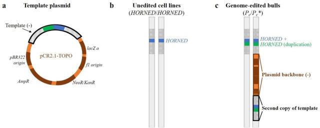
Here is what they claim happened (Fig 1): The template DNA is there, as evidenced by the PCR genotyping, but it inserted twice, with the rest of the plasmid in-between.

F1.large-5.jpg

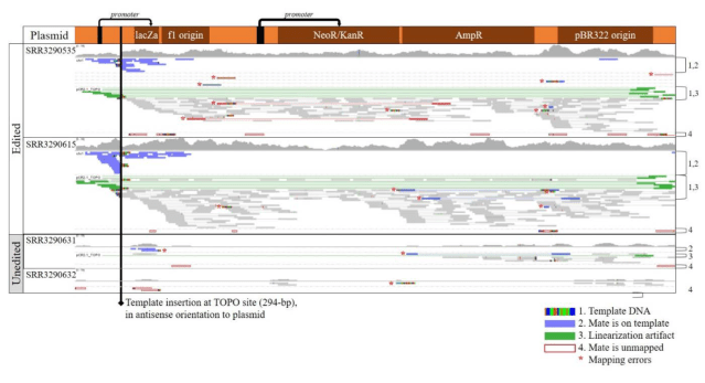
Here is the evidence (Supplementary figs 1 and 2): These are two annotated screenshots from IGV. The first shows alignments of reads from the calves and the unedited cell lines to the plasmid sequence. In the unedited cells, there are only stray reads, probably misplaced, but in the edited calves, ther are reads covering the plasmid throughout. Unless somehow else contaminated, this shows that the plasmid is somewhere in their genomes.

igv.png

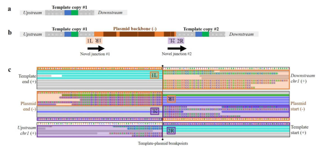
Where is it then? This second supplementary figure shows alignments to expected junctions: where template DNA and genome are supposed to join. The colourful letters are mismatches, showing where unexpected DNA shows up. This is the evidence for where the plasmid integrated and what kind of complex rearrangement of template, plasmid and genome happened at the cut site. This must have been found by looking at alignments, hypothesising an insertion, and looking for the junctions supporting it.

igv2.png

Why didn’t the PCR and targeted sequencing find this? As this third supplementary figure shows, the PCRs used could, theoretically, produce longer products including plasmid sequence. But they are way too long for regular PCR.

pcr.png

Looking at this picture, I wonder if there were a few attempts to make a primer pair that went from insert into the downstream sequence, that failed and got blamed on bad primer design or PCR conditions.

In summary, the 2019 preprint finds indirect evidence of the plasmid insertion by looking hard at short read alignments. Targeted sequencing or long read sequencing could give better evidence by observing he whole insertion. Recombinetics have acknowledged the problem, which makes me think that they’ve gone back to the DNA samples and checked.

Where does that leave us with quality control of gene editing? There are three kinds of problems to worry about:

  • Off-target edits in similar places in other parts of the genome; this seems to be what people used to worry about the most, and what Carlson & al checked for
  • Complex rearrangements around cut site (probably due to repeated cutting; this became a big concern after Kosicki & al (2018), and should apply both to on- and off-target cuts
  • Insertion of plasmid or mutated target; this is what happened in here

The ways people check gene edits (targeted Sanger sequencing and short read sequencing) doesn’t detect any of them particularly well, at least not without bespoke analysis. Maybe the kind of analysis that Norris & al do could be automated to some extent, but currently, the state of the art seems to be to manually look closely at alignments. If I was reviewing the preprint, I would have liked it if the manuscript had given a fuller description of how they arrived at this picture, and exactly what the evidence for this particular complex rearrangement is. This is a bit hard to follow.

Finally, is this embarrassing? On the one hand, this is important stuff, plasmid integration is a known problem, so the original researchers probably should have looked harder for it. On the other hand, the cell lines were edited and the clones born before a lot of the discussion and research of off-target edits and on-target rearrangements that came out of CRISPR being widely applied, and when long read sequencing was a lot less common. Maybe it was easier to think that the sort read off-target analysis was enough then. In any case, we need a solid way to quality check edits.

Literature

Molteni M. (2019) Brazil’s plan for gene edited-cows got scrapped–here’s why. Wired.

Carlson DF, et al. (2016) Production of hornless dairy cattle from genome-edited cell lines. Nature Biotechnology.

Norris AL, et al. (2019) Template plasmid integration in germline genome-edited cattle. BioRxiv.

Tan W, et al. (2013) Efficient nonmeiotic allele introgression in livestock using custom endonucleases. Proceedings of the National Academy of Sciences.

Bastiaansen JWM, et al. (2018) The impact of genome editing on the introduction of monogenic traits in livestock. Genetics Selection Evolution.

Kosicki M, Tomberg K & Bradley A. (2018) Repair of double-strand breaks induced by CRISPR–Cas9 leads to large deletions and complex rearrangements. Nature Biotechnology.

Journal club of one: ‘Biological relevance of computationally predicted pathogenicity of noncoding variants’

Wouldn’t it be great if we had a way to tell genetic variants that do something to gene function and regulation from those that don’t? This is a Really Hard Problem, especially for variants that fall outside of protein-coding regions, and thus may or may not do something to gene regulation.

There is a host of bioinformatic methods to tackle the problem, and they use different combinations of evolutionary analysis (looking at how often the position of the variant differs between or within species) and functional genomics (what histone modifications, chromatin accessibility etc are like at the location of the variant) and statistics (comparing known functional variants to other variants).

When a new method is published, it’s always accompanied by a receiver operating curve showing it predicting held-out data well, and some combination of comparisons to other methods and analyses of other datasets of known or presumed functional variants. However, one wonders how these methods will do when we use them to evaluate unknown variants in the lab, or eventually in the clinic.

This is what this paper, Liu et al (2019) Biological relevance of computationally predicted pathogenicity of noncoding variants is trying to do. They construct three test cases that are supposed to be more realistic (pessimistic) test beds for six noncoding variant effect predictors.

The tasks are:

  1. Find out which allele of a variant is the deleterious one. The presumed deleterious test alleles here are ones that don’t occur in any species of a large multiple genome alignment.
  2. Find a causative variant among a set of linked variants. The test alleles are causative variants from the Human Gene Mutation Database and some variants close to them.
  3. Enrich for causative variants among increasingly bigger sets of non-functional variants.

In summary, the methods don’t do too well. The authors think that they have ‘underwhelming performance’. That isn’t happy news, but I don’t think it’s such a surprise. Noncoding variant prediction is universally acknowledged to be tricky. In particular, looking at Task 3, the predictors are bound to look much less impressive in the face of class imbalance than in those receiver operating curves. Then again, class imbalance is going to be a fact when we go out to apply these methods to our long lists of candidate variants.

Task 1 isn’t that well suited to the tools, and the way it’s presented is a bit silly. After describing how they compiled their evolution-based test variant set, the authors write:

Our expectation was that a pathogenic allele would receive a significantly higher impact score (as defined for each of the six tested methods) than a non-pathogenic allele at the same position. Instead, we found that these methods were unsuccessful at this task. In fact, four of them (LINSIGHT, EIGEN, GWAVA, and CATO) reported identical scores for all alternative alleles at every position as they were not designed for allelic contrasts …

Sure, it’s hard to solve this problem with a program that only produces one score per site, but you knew that when you started writing this paragraph, didn’t you?

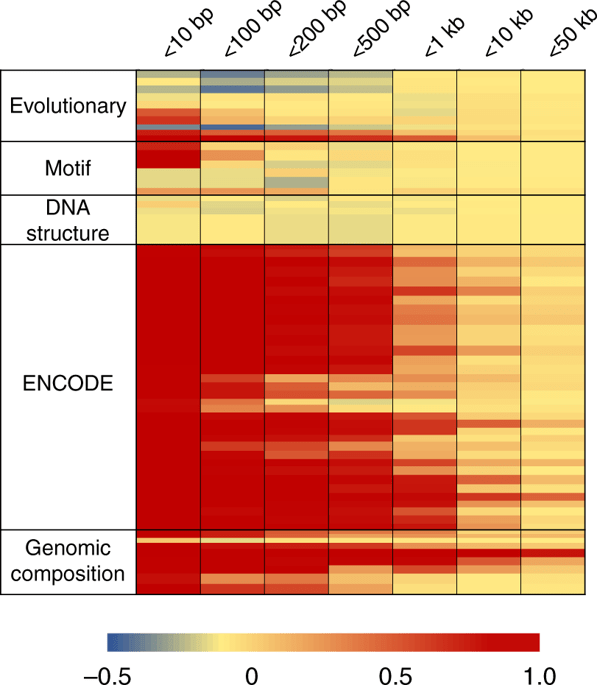
The whole paper is useful, but to me, the most interesting insight is that variants close to each other tend to have correlated features, meaning that there is little power to tell them apart (Task 2). This might be obvious if you think about it (e.g., if two variants fall in the same enhancer, how different can their chromatin state and histone modifications really be?), but I guess I haven’t thought that hard about it before. This high correlation is unfortunate, because that means that methods for finding causative variants (association and variant effect prediction) have poor spatial resolution. We might need something else to solve the fine mapping problem.

Figure 4 from Liu et al., showing correlation between features of linked variants.

Finally, shout-out to Reviewer 1 whose comment gave rise to these sentences:

An alternative approach is to develop a composite score that may improve upon individual methods. We examined one such method, namely PRVCS, which unfortunately had poor performance (Supplementary Figure 11).

I thought this read like something prompted by an eager beaver reviewer, and thanks to Nature Communications open review policy, we can confirm my suspicions. So don’t say that open review is useless.

Comment R1.d. Line 85: It would be interesting to see if a combination of the examined scores would better distinguish between pathogenic and non-pathogenic non-coding regions. Although we suspect there to be high correlation between features this will test the hypothesis that each score may not be sufficient on its own to make any distinction between pathogenic and non-pathogenic ncSNVs. However, a combined model might provide more discriminating power than individual scores, suggesting that each score captures part of the underlying information with regards to a region’s pathogenicity propensity.

Literature

Liu, L., Sanderford, M. D., Patel, R., Chandrashekar, P., Gibson, G., & Kumar, S. (2019). Biological relevance of computationally predicted pathogenicity of noncoding variants. Nature Communications, 10(1), 330.

Journal club of one: ‘The heritability fallacy’

Public debate about genetics often seems to centre on heritability and on psychiatric and mental traits, maybe because we really care about our minds, and because for a long time heritability was all human geneticists studying quantitative traits could estimate. Here is an anti-heritabililty paper that I think articulates many of the common grievances: Moore & Shenk (2016) The heritability fallacy. The abstract gives a snappy summary of the argument:

The term ‘heritability,’ as it is used today in human behavioral genetics, is one of the most misleading in the history of science. Contrary to popular belief, the measurable heritability of a trait does not tell us how ‘genetically inheritable’ that trait is. Further, it does not inform us about what causes a trait, the relative influence of genes in the development of a trait, or the relative influence of the environment in the development of a trait. Because we already know that genetic factors have significant influence on the development of all human traits, measures of heritability are of little value, except in very rare cases. We, therefore, suggest that continued use of the term does enormous damage to the public understanding of how human beings develop their individual traits and identities.

At first glance, this paper should be a paper for me. I tend to agree that heritability estimates of human traits aren’t very useful. I also agree that geneticists need to care about the interpretations of their claims beyond the purely scientific domain. But the more I read, the less excited I became. The paper is a list of complaints about heritability coefficients. Some are more or less convincing. For example, I find it hard to worry too much about the ‘equal environments assumption’ in twin studies. But sure, it’s hard to identify variance components, and in practice, researchers sometimes restort to designs that are a lot iffier than twin studies.

But I think the main thrust of the paper is this huge overstatement:

Most important of all is a deep flaw in an assumption that many people make about biology: That genetic influences on trait development can be separated from their environmental context. However, contemporary biology has demonstrated beyond any doubt that traits are produced by interactions between genetic and nongenetic factors that occur in each moment of developmental time … That is to say, there are simply no such things as gene-only influences.

There certainly is such a thing as additive genetic variance as well as additive gene action. This passage only makes sense to me if ‘interaction’ is interpreted not as a statistical term but as describing a causal interplay. If so, it is perfectly true that all traits are the outcomes of interplay between genes and environment. It doesn’t follow that genetic variants in populations will interact with variable environments to the degree that quantitative genetic models are ‘nonsensical in most circumstances’.

They illustrate with this parable: Billy and Suzy are filling a bucket. Suzy is holding the hose and Billy turns on the tap. How much of the water is due to Billy and how much is due to Suzy? The answer is supposed to be that the question makes no sense, because they are both filling the bucket through a causal interplay. Well. If they’re filling a dozen buckets, and halfway through, Billy opens the tap half a turn more, and Suzy starts moving faster between buckets, because she’s tired of this and wants lunch … The correct level of analysis for the quantitative bucketist isn’t Billy, Suzy and the hose. It is the half-turn of the tap and Suzy’s moving of the nozzle.

The point is that quantitative genetic models describe variation between individuals. The authors know this, of course, but they write as if genetic analysis of variance is some kind of sleight of hand, as if quantitative genetics ought to be about development, and the fact that it isn’t is a deliberate obfuscation. Here is how they describe Jay Lush’s understanding of heritability:

The intention was ‘to quantify the level of predictability of passage of a biologically interesting phenotype from parent to offspring’. In this way, the new technical use of ‘heritability’ accurately reflected that period’s understanding of genetic determinism. Still, it was a curious appropriation of the term, because—even by the admission of its proponents—it was meant only to represent how variation in DNA relates to variation in traits across a population, not to be a measure of the actual influence of genes on the development of any given trait.

I have no idea what position Lush took on genetic determinism. But we can find the context of heritability by looking at the very page before in Animal breeding plans. The definition of the heritability coefficient occurs on page 87. This is how Lush starts the chapter on page 86:

In the strictest sense of the word, the question of whether a characteristic is hereditary or environmental has no meaning. Every characteristic is both hereditary and environmental, since it is the end result of a long chain of interactions of the genes with each other, with the environment and with the intermediate products at each stage of development. The genes cannot develop the characteristic unless they have the proper environment, and no amount of attention to the environment will cause the characteristc to develop unless the necessary genes are present. If either the genes or the environment are changed, the characteristic which results from their interactions may be changed.

I don’t know — maybe the way quantitative genetics has been used in human behavioural and psychiatric genetics invites genetic determinism. Or maybe genetic determinism is one of those false common-sense views that are really hard to unlearn. In any case, I don’t think it’s reasonable to put the blame on the concept of heritability for not being some general ‘measure of the biological inheritability of complex traits’ — something that it was never intended to be, and cannot possibly be.

My guess is that new debates will be about polygenic scores and genomic prediction. I hope that will be more useful.

Literature

David S. Moore & David Shenk (2016) The heritability fallacy

Jay Lush Animal breeding plans. Online at: https://archive.org/details/animalbreedingpl032391mbp/page/n99

Journal club of one: ‘Sacred text as cultural genome: an inheritance mechanism and method for studying cultural evolution’

This is a fun paper about something I don’t know much about: Hartberg & Sloan Wilson (2017) ‘Sacred text as cultural genome: an inheritance mechanism and method for studying cultural evolution‘. It does exactly what it says on the package: it takes an image from genome science, that of genomic DNA and gene expression, and uses it as a metaphor for how pastors in Christian churches use the Bible. So, the Bible is the genome, churches are cells, and citing bible passages in a sermon is gene expression–at least something along those lines.

The authors use a quantitative analysis analogous to differential gene expression to compare the Bible passages cited in sermons from six Protestant churches in the US with different political leanings (three conservative and three progressive; coincidentally, N = 3 is kind of the stereotypical sample size of an early 2000s gene expression study). The main message is that the churches use the Bible differently, that the conservative churches use more of the text, and that even when they draw on the same book, they use different verses.

They exemplify with Figure 3, which shows a ‘Heat map showing the frequency with which two churches, one highly conservative (C1) and one highly progressive (P1), cite specific verses within chapter 3 of the Gospel According to John in their Sunday sermons.’ I will not reproduce it for copyright reasons, but it pretty clearly shows how P1 often cites the first half of the chapter but doesn’t use the second half at all. C1, instead, uses verses from the whole chapter, but its three most used verses are all in latter half, that is the block that P1 doesn’t use at all. What are these verses? The paper doesn’t quote them except 3:16 ‘For God so loved the world, that he gave his one and only Son, that whoever believes in him should not perish, but have eternal life’, which is the exception to the pattern — it’s the most common verse in both churches (and generally, a very famous passage).

Chapter 3 of the Gospel of John is the story of how Jesus teaches Nicodemus. Here is John 3:1-17:

1 Now there was a man of the Pharisees named Nicodemus, a ruler of the Jews. 2 The same came to him by night, and said to him, ”Rabbi, we know that you are a teacher come from God, for no one can do these signs that you do, unless God is with him.”
3 Jesus answered him, ”Most certainly, I tell you, unless one is born anew, he can’t see God’s Kingdom.”
4 Nicodemus said to him, ”How can a man be born when he is old? Can he enter a second time into his mother’s womb, and be born?”
5 Jesus answered, ”Most certainly I tell you, unless one is born of water and spirit, he can’t enter into God’s Kingdom. 6 That which is born of the flesh is flesh. That which is born of the Spirit is spirit. 7 Don’t marvel that I said to you, ‘You must be born anew.’ 8 The wind blows where it wants to, and you hear its sound, but don’t know where it comes from and where it is going. So is everyone who is born of the Spirit.”
9 Nicodemus answered him, ”How can these things be?”
10 Jesus answered him, ”Are you the teacher of Israel, and don’t understand these things? 11 Most certainly I tell you, we speak that which we know, and testify of that which we have seen, and you don’t receive our witness. 12 If I told you earthly things and you don’t believe, how will you believe if I tell you heavenly things? 13 No one has ascended into heaven but he who descended out of heaven, the Son of Man, who is in heaven. 14 As Moses lifted up the serpent in the wilderness, even so must the Son of Man be lifted up, 15 that whoever believes in him should not perish, but have eternal life. 16 For God so loved the world, that he gave his one and only Son, that whoever believes in him should not perish, but have eternal life. 17 For God didn’t send his Son into the world to judge the world, but that the world should be saved through him.”

This is the passage that P1 uses a lot, but they break before they get to the verses that come right after: John 3:18-21. The conservative church uses them the most out of this chapter.

18 Whoever believes in him is not condemned, but whoever does not believe stands condemned already because they have not believed in the name of God’s one and only Son. 19 This is the verdict: Light has come into the world, but people loved darkness instead of light because their deeds were evil. 20 Everyone who does evil hates the light, and will not come into the light for fear that their deeds will be exposed. 21 But whoever lives by the truth comes into the light, so that it may be seen plainly that what they have done has been done in the sight of God.

So this is consistent with the idea of the paper: In the progressive church, the pastor emphasises the story about doubt and the possibility of salvation, where Nicodemus comes to ask Jesus for explanations, and Jesus talks about being born again. It also has some beautiful perplexing Jesus-style imagery with the spirit being like the wind. In the conservative church, the part about condemnation and evildoers hating the light gets more traction.

As for the main analogy between the Bible and a genome, I’m not sure that it works. The metaphors are mixed, and it’s not obvious what the unit of inheritance is. For example, when the paper talks about ‘fitness-enhanching information’, does that refers to the fitness of the church, the members of the church, or the Bible itself? The paper sometimes talk as if the bible was passed on from generation to generation, for instance here in the introduction:

Any mechanism of inheritance must transmit information across generations with high fidelity and translate this information into phenotypic expression during each generation. In this article we argue that sacred texts have these properties and therefore qualify as important inheritance mechanisms in cultural evolution.

But the sacred text isn’t passed on from generation to generation. The Bible is literally a book that is transmitted by printing. What may be passed on is the way pastors interpret it and, in the authors’ words, ‘cherry pick’ verses to cite. But clearly, that is not stored in the bible ‘genome’ but somehow in the culture of churches and the institutions of learning that pastors attend.

If we want to stick to the idea of the bible as a genome, I think this story makes just as much sense: Don’t think about how this plasticity of interpretation may be adaptive for humans. Instead, take a sacred text-centric perspective, analogous to the gene-centric perspective. Think of the plasticity in interpretation as preserving the fitness of the bible by making it fit community values. Because the Bible can serve as source materials for churches with otherwise different values, it survives as one of the most important and widely read books in the world.

Literature

Hartberg, Yasha M., and David Sloan Wilson. ”Sacred text as cultural genome: an inheritance mechanism and method for studying cultural evolution.” Religion, Brain & Behavior 7.3 (2017): 178-190.

The Bible quotes are from the World English Bible translation.