”Locus” is one of those confusing genetics terms (its meaning, not just its pronunciation). We can probably all agree with a dictionary and with Wikipedia that it means a place in the genome, but a place of what and in what sense? We also use place-related word like ”site” and ”region” that one might think were synonymous, but don’t seem to be.
For an example, we can look at this relatively recent preprint (Chebib & Guillaume 2020) about a model of the causes of genetic correlation. They have pairs of linked loci that each affect one trait each (that’s the tight linkage condition), and also a set of loci that affect both traits (the pleiotropic condition), correlated Gaussian stabilising selection, and different levels of mutation, migration and recombination between the linked pairs. A mutation means adding a number to the effect of an allele.
This means that loci in this model can have a large number of alleles with quantitatively different effects. The alleles at a locus share a distribution of mutation effects, that can be either two-dimensional (with pleiotropy) or one-dimensional. They also share a recombination rate with all other loci, which is constant.
What kind of DNA sequences can have these properties? Single nucleotide sites are out of the question, as they can have four, or maybe five alleles if you count a deletion. Larger structural variants, such as inversions or allelic series of indels might work. A protein-coding gene taken as a unit could have a huge number of different alleles, but they would probably have different distributions of mutational effects in different sites, and (relatively small) differences in genetic distance to different sites.
It seems to me that we’re talking about an abstract group of potential alleles that have sufficiently similar effects and that are sufficiently closely linked. This is fine; I’m not saying this to criticise the model, but to explore how strange a locus really is.
They find that there is less genetic correlation with linkage than with pleiotropy, unless the mutation rate is high, which leads to a discussion about mutation rate. This reasoning about the mutation rate of a locus illustrates the issue:
A high rate of mutation (10−3) allows for multiple mutations in both loci in a tightly linked pair to accumulate and maintain levels of genetic covariance near to that of mutations in a single pleiotropic locus, but empirical estimations of mutation rates from varied species like bacteria and humans suggests that per-nucleotide mutation rates are in the order of 10−8 to 10−9 … If a polygenic locus consists of hundreds or thousands of nucleotides, as in the case of many quantitative trait loci (QTLs), then per-locus mutation rates may be as high as 10−5, but the larger the locus the higher the chance of recombination between within-locus variants that are contributing to genetic correlation. This leads us to believe that with empirically estimated levels of mutation and recombination, strong genetic correlation between traits are more likely to be maintained if there is an underlying pleiotropic architecture affecting them than will be maintained due to tight linkage.
I don’t know if it’s me or the authors who are conceptually confused here. If they are referring to QTL mapping, it is true that the quantitative trait loci that we detect in mapping studies often are huge. ”Thousands of nucleotides” is being generous to mapping studies: in many cases, we’re talking millions of them. But the size of a QTL region from a mapping experiment doesn’t tell us how many nucleotides in it that matter to the trait. It reflects our poor resolution in delineating the, one or more, causative variants that give rise to the association signal. That being said, it might be possible to use tricks like saturation mutagenesis to figure out which mutations within a relevant region that could affect a trait. Then, we could actually observe a locus in the above sense.
Another recent theoretical preprint (Chantepie & Chevin 2020) phrases it like this:
[N]ote that the nature of loci is not explicit in this model, but in any case these do not represent single nucleotides or even genes. Rather, they represent large stretches of effectively non-recombining portions of the genome, which may influence the traits by mutation. Since free recombination is also assumed across these loci (consistent with most previous studies), the latter can even be thought of as small chromosomes, for which mutation rates of the order to 10−2 seem reasonable.
Literature
Chebib and Guillaume. ”Pleiotropy or linkage? Their relative contributions to the genetic correlation of quantitative traits and detection by multi-trait GWA studies.” bioRxiv (2019): 656413.
Chantepie and Chevin. ”How does the strength of selection influence genetic correlations?” bioRxiv (2020).
 ,
,  and
and  before selection.
 for Aa and
  for aa. We can think of this as the probability of contributing to the next generation.
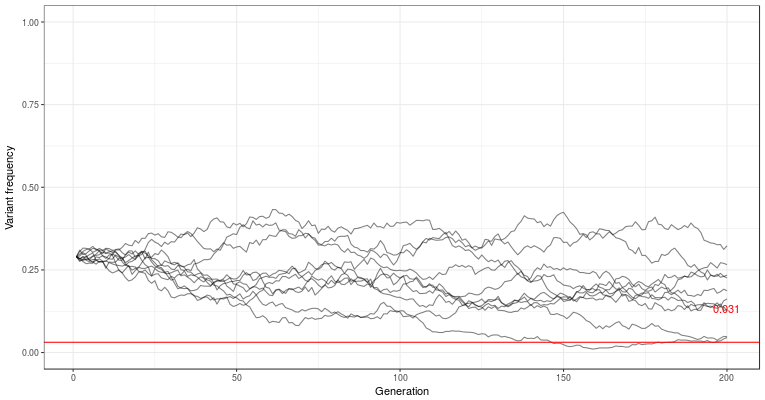
 is the mutation rate. It’s not easy to see what is going on here, but we can draw it in the graph, and see that it’s usually very small. In these small populations, where drift is a major player, the variants are often completely lost, or drift to higher frequency by chance.