”Dangerous gene myths abound”

Philip Ball, who is a knowledgeable and thoughtful science writer, published an piece in the Guardian a couple of months ago about the misunderstood legacy of the human genome project: ”20 years after the human genome was first sequenced, dangerous gene myths abound”.

The human genome project published the draft reference genome for the human species 20 years ago. Ball argues, in short, that the project was oversold with promises that it couldn’t deliver, and consequently has not delivered. Instead, the genome project was good for other things that had more to do with technology development and scientific infrastructure. The sequencing of the human genome was the platform for modern genome science, but it didn’t, for example, cure cancer or uncover a complete set of instructions for building a human.

He also argues that the rhetoric of human genome hype, which did not end with the promotion of the human genome project (see the ENCODE robot punching cancer in the face, for example), is harmful. It is scientifically harmful because it oversimplifies modern genetics, and it is politically harmful because it aligns well with genetic determinism and scientific racism.

I believe Ball is entirely right about this.

Selling out

The breathless hype around the human genome project was embarrassing. Ball quotes some fragments, but you can to to the current human genome project site and enjoy quotes like ”it’s a transformative textbook of medicine, with insights that will give health care providers immense new powers to treat, prevent and cure disease”. This image has some metonymical truth to it — human genomics is helping medical science in different ways — but even as a metaphor, it is obviously false. You can go look at the human reference genome if you want, and you will discover that the ”text” such as it is looks more like this than a medical textbook:

TTTTTTTTCCTTTTTTTTCTTTTGAGATGGAGTCTCGCTCTGCCGCCCAGGCTGGAGTGC
AGTAGCTCGATCTCTGCTCACTGCAAGCTCCGCCTCCCGGGTTCACGCCATTCTCCTGCC
TCAGCCTCCTGAGTAGCTGGGACTACAGGCGCCCACCACCATGCCCAGCTAATTTTTTTT
TTTTTTTTTTTGGTATTTTTAGTAGAGACGGGGTTTCACCGTGTTAGCCAGGATGGTCTC
AATCTCCTGACCTTGTGATCCGCCCGCCTCGGCCTCCCACAGTGCTGGGATTACAGGC

This is a human Alu element from chromosome 17. It’s also in an intron of a gene, flanking a promoter, a few hundred basepairs away from an insulator (see the Ensembl genome browser) … All that is stuff that cannot be read from the sequence alone. You might be able to tell that it’s Alu if you’re an Alu genius or run a sequence recognition software, but there is no to read the other contextual genomic information, and there is no way you can tell anything about human health by reading it.

I think Ball is right that this is part of simplistic genetics that doesn’t appreciate the complexity either quantitative or molecular genetics. In short, quantitative genetics, as a framework, says that inheritance of traits between relatives is due to thousands and thousands of genetic differences each of them with tiny effects. Molecular genetics says that each of those genetic differences may operate through any of a dizzying selection of Rube Goldberg-esque molecular mechanisms, to the point where understanding one of them might be a lifetime of laboratory investigation.

Simple inheritance is essentially a fiction, or put more politely: a simple model that is useful as a step to build up a more better picture of inheritance. This is not knew; the knowledge that everything of note is complex has been around since the beginning of genetics. Even rare genetic diseases understood as monogenic are caused by sometimes thousands of different variants that happen in a particular small subset of the genome. Really simple traits, in the sense of one variant–one phenotype, seldom happen in large mixing and migrating populations like humans; they may occur in crosses constructed in the lab, or in extreme structured populations like dog breeds or possibly with balancing selection.

Can you market thick sequencing?

Ball is also right about what it was most useful about the human genome project: it enabled research at scale into human genetic variation, and it stimulated development of sequencing methods, both generating and using DNA sequence. Lowe (2018) talks about ”thick” sequencing, a notion of sequencing that includes associated activities like assembly, annotation and distribution to a community of researchers — on top of ”thin” sequencing as determination of sequences of base pairs. Thick sequencing better captures how genome sequencing is used and stimulates other research, and aligns with how sequencing is an iterative process, where reference genomes are successively refined and updated in the face of new data, expert knowledge and quality checking.

It is hard to imagine gene editing like CRISPR being applied in any human cell without a good genome sequence to help find out what to cut out and what to put instead. It is hard to imagine the developments in functional genomics that all use short read sequencing as a read-out without having a good genome sequence to anchor the reads on. It is possible to imagine genome-wide association just based on very dense linkage maps, but it is a bit far-fetched. And so on.

Now, this raises a painful but interesting question: Would the genome project ever have gotten funded on reasonable promises and reasonable uncertainties? If not, how do we feel about the genome hype — necessary evil, unforgivable deception, something in-between? Ball seems to think that gene hype was an honest mistake and that scientists were surprised that genomes turned out to be more complicated than anticipated. Unlike him, I do not believe that most researchers honestly believed the hype — they must have known that they were overselling like crazy. They were no fools.

An example of this is the story about how many genes humans have. Ball writes:

All the same, scientists thought genes and traits could be readily matched, like those children’s puzzles in which you trace convoluted links between two sets of items. That misconception explains why most geneticists overestimated the total number of human genes by a factor of several-fold – an error typically presented now with a grinning “Oops!” rather than as a sign of a fundamental error about what genes are and how they work.

This is a complicated history. Gene number estimates are varied, but enjoy this passage from Lewontin in 1977:

The number of genes is not large

While higher organisms have enough DNA to specify from 100,000 to 1,000,000 proteins of average size, it appears that the actual number of cistrons does not exceed a few thousand. Thus, saturation lethal mapping of the fourth chromosome (Hochman, 1971) and the X chromosome (Judd, Shen and Kaufman, 1972) of Drosophila melanogbaster make it appear that there is one cistron per salivary chromosome band, of which there are 5,000 in this species. Whether 5,000 is a large or small number of total genes depends, of course, on the degree of interaction of various cistrons in influencing various traits. Nevertheless, it is apparent that either a given trait is strongly influenced by only a small number of genes, or else there is a high order of gene interactions among developmental systems. With 5,000 genes we cannot maintain a view that different parts of the organism are both independent genetically and each influenced by large number of gene loci.

I don’t know if underestimating by an few folds is worse than overestimating by a few folds (D. melanogaster has 15,000 protein-coding genes or so), but the point is that knowledgeable geneticists did not go around believing that there was a simple 1-to-1 mapping between genes and traits, or even between genes and proteins at this time. I know Lewontin is a population geneticist, and in the popular mythology population geneticists are nothing but single-minded bean counters who do not appreciate the complexity of molecular biology … but you know, they were no fools.

The selfish cistron

One thing Ball gets wrong is evolutionary genetics, where he mixes genetic concepts that, really, have very little to do with each other despite superficially sounding similar.

Yet plenty remain happy to propagate the misleading idea that we are “gene machines” and our DNA is our “blueprint”. It is no wonder that public understanding of genetics is so blighted by notions of genetic determinism – not to mention the now ludicrous (but lucrative) idea that DNA genealogy tells you which percentage of you is “Scots”, “sub-Saharan African” or “Neanderthal”.

This passage smushes two very different parts of genetics together, that don’t belong together and have nothing to do with with the preceding questions about how many genes there are or if the DNA is a blueprint: The gene-centric view of adaptation, a way of thinking of natural selection where you imagine genetic variants (not organisms, not genomes, not populations or species) as competing for reproduction; and genetic genealogy and ancestry models, where you describe how individuals are related based on the genetic variation they carry. The gene-centric view is about adaptation, while genetic genealogy works because of effectively neutral genetics that just floats around, giving us a unique individual barcode due to the sheer combinatorics.

He doesn’t elaborate on the gene machines, but it links to a paper (Ridley 1984) on Williams’ and Dawkins’ ”selfish gene” or ”gene-centric perspective”. I’ve been on about this before, but when evolutionary geneticists say ”selfish gene”, they don’t mean ”the selfish protein-coding DNA element”; they mean something closer to ”the selfish allele”. They are not committed to any view that the genome is a blueprint, or that only protein-coding genes matter to adaptation, or that there is a 1-to-1 correspondence between genetic variants and traits.

This is the problem with correcting misconceptions in genetics: it’s easy to chide others for being confused about the parts you know well, and then make a hash of some other parts that you don’t know very well yourself. Maybe when researchers say ”gene” in a context that doesn’t sound right to you, they have a different use of the word in mind … or they’re conceptually confused fools, who knows.

Literature

Lewontin, R. C. (1977). The relevance of molecular biology to plant and animal breeding. In International Conference on Quantitative Genetics. Ames, Iowa (USA). 16-21 Aug 1976.

Lowe, J. W. (2018). Sequencing through thick and thin: Historiographical and philosophical implications. Studies in History and Philosophy of Science Part C: Studies in History and Philosophy of Biological and Biomedical Sciences, 72, 10-27.

A model of polygenic adaptation in an infinite population

How do allele frequencies change in response to selection? Answers to that question include ”it depends”, ”we don’t know”, ”sometimes a lot, sometimes a little”, and ”according to a nonlinear differential equation that actually doesn’t look too horrendous if you squint a little”. Let’s look at a model of the polygenic adaptation of an infinitely large population under stabilising selection after a shift in optimum. This model has been developed by different researchers over the years (reviewed in Jain & Stephan 2017).

Here is the big equation for allele frequency change at one locus:

\dot{p}_i = -s \gamma_i p_i q_i (c_1 - z') - \frac{s \gamma_i^2}{2} p_i q_i (q_i - p_i) + \mu (q_i - p_i )

That wasn’t so bad, was it? These are the symbols:

  • the subscript i indexes the loci,
  • \dot{p} 
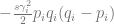
is the change in allele frequency per time,
  • \gamma_i is the effect of the locus on the trait (twice the effect of the positive allele to be precise),
  • p_i is the frequency of the positive allele,
  • q_i the frequency of the negative allele,
  • s is the strength of selection,
  • c_1 is the phenotypic mean of the population; it just depends on the effects and allele frequencies
  • \mu is the mutation rate.

This breaks down into three terms that we will look at in order.

The directional selection term

-s \gamma_i p_i q_i (c_1 - z')

is the term that describes change due to directional selection.

Apart from the allele frequencies, it depends on the strength of directional selection s, the effect of the locus on the trait \gamma_i and how far away the population is from the new optimum (c_1 - z'). Stronger selection, larger effect or greater distance to the optimum means more allele frequency change.

It is negative because it describes the change in the allele with a positive effect on the trait, so if the mean phenotype is above the optimum, we would expect the allele frequency to decrease, and indeed: when

(c_1 - z') < 0

this term becomes negative.

If you neglect the other two terms and keep this one, you get Jain & Stephan's "directional selection model", which describes behaviour of allele frequencies in the early phase before the population has gotten close to the new optimum. This approximation does much of the heavy lifting in their analysis.

The stabilising selection term

-\frac{s \gamma_i^2}{2} p_i q_i (q_i - p_i)

is the term that describes change due to stabilising selection. Apart from allele frequencies, it depends on the square of the effect of the locus on the trait. That means that, regardless of the sign of the effect, it penalises large changes. This appears to make sense, because stabilising selection strives to preserve traits at the optimum. The cubic influence of allele frequency is, frankly, not intuitive to me.

The mutation term

Finally,

\mu (q_i - p_i )

is the term that describes change due to new mutations. It depends on the allele frequencies, i.e. how of the alleles there are around that can mutate into the other alleles, and the mutation rate. To me, this is the one term one could sit down and write down, without much head-scratching.

Walking in allele frequency space

Jain & Stephan (2017) show a couple of examples of allele frequency change after the optimum shift. Let us try to draw similar figures. (Jain & Stephan don’t give the exact parameters for their figures, they just show one case with effects below their threshold value and one with effects above.)

First, here is the above equation in R code:

pheno_mean <- function(p, gamma) {
  sum(gamma * (2 * p - 1))
}

allele_frequency_change <- function(s, gamma, p, z_prime, mu) {
  -s * gamma * p * (1 - p) * (pheno_mean(p, gamma) - z_prime) +
    - s * gamma^2 * 0.5 * p * (1 - p) * (1 - p - p) +
    mu * (1 - p - p)
}

With this (and some extra packaging; code on Github), we can now plot allele frequency trajectories such as this one, which starts at some arbitrary point and approaches an optimum:

Animation of alleles at two loci approaching an equilibrium. Here, we have two loci with starting frequencies 0.2 and 0.1 and effect size 1 and 0.01, and the optimum is at 0. The mutation rate is 10-4 and the strength of selection is 1. Animation made with gganimate.

Resting in allele frequency space

The model describes a shift from one optimum to another, so we want want to start at equilibrium. Therefore, we need to know what the allele frequencies are at equilibrium, so we solve for 0 allele frequency change in the above equation. The first term will be zero, because

(c_1 - z') = 0

when the mean phenotype is at the optimum. So, we can throw away that term, and factor the rest equation into:

(1 - 2p) (-\frac{s \gamma ^2}{2} p(1-p) + \mu) = 0

Therefore, one root is p = 1/2
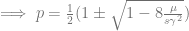
. Depending on your constitution, this may or may not be intuitive to you. Imagine that you have all the loci, each with a positive and negative allele with the same effect, balanced so that half the population has one and the other half has the other. Then, there is this quadratic equation that gives two other equilibria:

\mu - \frac{s\gamma^2}{2}p(1-p) = 0
\implies p = \frac{1}{2} (1 \pm \sqrt{1 - 8 \frac{\mu}{s \gamma ^2}})

These points correspond to mutation–selection balance with one or the other allele closer to being lost. Jain & Stephan (2017) show a figure of the three equilibria that looks like a semicircle (from the quadratic equation, presumably) attached to a horizontal line at 0.5 (their Figure 1). Given this information, we can start our loci out at equilibrium frequencies. Before we set them off, we need to attend to the effect size.

How big is a big effect? Hur långt är ett snöre?

In this model, there are big and small effects with qualitatively different behaviours. The cutoff is at:

\hat{\gamma} = \sqrt{ \frac{8 \mu}{s}}

If we look again at the roots to the quadratic equation above, they can only exist as real roots if

\frac {8 \mu}{s \gamma^2} < 1

because otherwise the expression inside the square root will be negative. This inequality can be rearranged into:

\gamma^2 > \frac{8 \mu}{s}

This means that if the effect of a locus is smaller than the threshold value, there is only one equilibrium point, and that is at 0.5. It also affects the way the allele frequency changes. Let us look at two two-locus cases, one where the effects are below this threshold and one where they are above it.

threshold <- function(mu, s) sqrt(8 * mu / s)

threshold(1e-4, 1)
[1] 0.02828427

With mutation rate of 10-4 and strength of selection of 1, the cutoff is about 0.028. Let our ”big” loci have effect sizes of 0.05 and our small loci have effect sizes of 0.01, then. Now, we are ready to shift the optimum.

The small loci will start at an equilibrium frequency of 0.5. We start the large loci at two different equilibrium points, where one positive allele is frequent and the other positive allele is rare:

get_equilibrium_frequencies <- function(mu, s, gamma) {
  c(0.5,
    0.5 * (1 + sqrt(1 - 8 * mu / (s * gamma^2))),
    0.5 * (1 - sqrt(1 - 8 * mu / (s * gamma^2))))
}

(eq0.05 <- get_equilibrium_frequencies(1e-4, 1, 0.05))
[1] 0.50000000 0.91231056 0.08768944
get_equlibrium_frequencies(1e-4, 1, 0.01)
[1] 0.5 NaN NaN

Look at them go!

These animations show the same qualitative behaviour as Jain & Stephan illustrate in their Figure 2. With small effects, there is gradual allele frequency change at both loci:

However, with large effects, one of the loci (the one on the vertical axis) dramatically changes in allele frequency, that is it’s experiencing a selective sweep, while the other one barely changes at all. And the model will show similar behaviour when the trait is properly polygenic, with many loci, as long as effects are large compared to the (scaled) mutation rate.

Here, I ran 10,000 time steps; if we look at the phenotypic means, we can see that they still haven’t arrived at the optimum at the end of that time. The mean with large effects is at 0.089 (new optimum of 0.1), and the mean with small effects is 0.0063 (new optimum: 0.02).

Let’s end here for today. Maybe another time, we can return how this model applies to actually polygenic architectures, that is, with more than two loci. The code for all the figures is on Github.

Literature

Jain, K., & Stephan, W. (2017). Modes of rapid polygenic adaptation. Molecular biology and evolution, 34(12), 3169-3175.

Excerpts about genomics in animal breeding

Here are some good quotes I’ve come across while working on something.

Artificial selection on the phenotypes of domesticated species has been practiced consciously or unconsciously for millennia, with dramatic results. Recently, advances in molecular genetic engineering have promised to revolutionize agricultural practices. There are, however, several reasons why molecular genetics can never replace traditional methods of agricultural improvement, but instead they should be integrated to obtain the maximum improvement in economic value of domesticated populations.

Lande R & Thompson R (1990) Efficiency of marker-assisted selection in the improvement of quantitative traits. Genetics.

Smith and Smith suggested that the way to proceed is to map QTL to low resolution using standard mapping methods and then to increase the resolution of the map in these regions in order to locate more closely linked markers. In fact, future developments should make this approach unnecessary and make possible high resolution maps of the whole genome, even, perhaps, to the level of the DNA sequence. In addition to easing the application of selection on loci with appreciable individual effects, we argue further that the level of genomic information available will have an impact on infinitesimal models. Relationship information derived from marker information will replace the standard relationship matrix; thus, the average relationship coefficients that this represents will be replaced by actual relationships. Ultimately, we can envisage that current models combining few selected QTL with selection on polygenic or infinitesimal effects will be replaced with a unified model in which different regions of the genome are given weights appropriate to the variance they explain.

Haley C & Visscher P. (1998) Strategies to utilize marker–quantitative trait loci associations. Journal of Dairy Science.

Instead, since the late 1990s, DNA marker genotypes were included into the conventional BLUP analyses following Fernando and Grossman (1989): add the marker genotype (0, 1, or 2, for an animal) as a fixed effect to the statistical model for a trait, obtain the BLUP solutions for the additive polygenic effect as before, and also obtain the properly adjusted BLUE solution for the marker’s allele substitution effect; multiply this BLUE by 0, 1, or 2 (specic for the animal) and add the result to the animal’s BLUP to obtain its marker-enhanced EBV. A logical next step was to treat the marker genotypes as semi-random effects, making use of several different shrinkage strategies all based on the marker heritability (e.g., Tsuruta et al., 2001); by 2007, breeding value estimation packages such as PEST (Neumaier and Groeneveld, 1998) supported this strategy as part of their internal calculations. At that time, a typical genetic evaluation run for a production trait would involve up to 30 markers.

Knol EF, Nielsen B, Knap PW. (2016) Genomic selection in commercial pig breeding. Animal Frontiers.

Although it has not caught the media and public imagination as much as transgenics and cloning, genomics will, I believe, have just as great a long-term impact. Because of the availability of information from genetically well-researched species (humans and mice), genomics in farm animals has been established in an atypical way. We can now see it as progressing in four phases: (i) making a broad sweep map (~20 cM) with both highly informative (microsatellite) and evolutionary conserved (gene) markers; (ii) using the informative markers to identify regions of chromosomes containing quantitative trait loci (QTL) controlling commercially important traits–this requires complex pedigrees or crosses between phenotypically anc genetically divergent strains; (iii) progressing from the informative markers into the QTL and identifying trait genes(s) themselves either by complex pedigrees or back-crossing experiments, and/or using the conserved markers to identify candidate genes from their position in the gene-rich species; (iv) functional analysis of the trait genes to link the genome through physiology to the trait–the ‘phenotype gap’.

Bulfield G. (2000) Biotechnology: advances and impact. Journal of the Science of Food and Agriculture.

I believe animal breeding in the post-genomic era will be dramatically different to what it is today. There will be massive research effort to discover the function of genes including the effect of DNA polymorphisms on phenotype. Breeding programmes will utilize a large number of DNA-based tests for specific genes combined with new reproductive techniques and transgenes to increase the rate of genetic improvement and to produce for, or allocate animals to, the product line to which they are best suited. However, this stage will not be reached for some years by which time many of the early investors will have given up, disappointed with the early benefits.

Goddard M. (2003). Animal breeding in the (post-) genomic era. Animal Science.

Genetics is a quantitative subject. It deals with ratios, with measurements, and with the geometrical relationships of chromosomes. Unlike most sciences that are based largely on mathematical techniques, it makes use of its own system of units. Physics, chemistry, astronomy, and physiology all deal with atoms, molecules, electrons, centimeters, seconds, grams–their measuring systems are all reducible to these common units. Genetics has none of these as a recognizable component in its fundamental units, yet it is a mathematically formulated subject that is logically complete and self-contained.

Sturtevant AH & Beadle GW. (1939) An introduction to genetics. W.B. Saunders company, Philadelphia & London.

We begin by asking why genes on nonhomologous chromosomes assort independently. The simple cytological story rehearsed above answers the questions. That story generates further questions. For example, we might ask why nonhomologous chromosomes are distributed independently at meiosis. To answer this question we could describe the formation of the spindle and the migration of chromosomes to the poles of the spindle just before meiotic division. Once again, the narrative would generate yet further questions. Why do the chromosomes ”condense” at prophase? How is the spindle formed? Perhaps in answering these questions we would begin to introduce the chemical details of the process. Yet simply plugging a molecular account into the narratives offered at the previous stages would decrease the explanatory power of those narratives.

Kitcher, P. (1984) 1953 and all that. A tale of two sciences. Philosophical Review.

And, of course, this great quote by Jay Lush.

There is no breeder’s equation for environmental change

This post is about why heritability coefficients of human traits can’t tell us what to do. Yes, it is pretty much an elaborate subtweet.

Let us begin in a different place, where heritability coefficients are useful, if only a little. Imagine there is selection going on. It can be natural or artificial, but it’s selection the old-fashioned way: there is some trait of an individual that makes it more or less likely to successfully reproduce. We’re looking at one generation of selection: there is one parent generation, some of which reproduce and give rise to the offspring generation.

Then, if we have a well-behaved quantitative trait, no systematic difference between the environments that the two generations experience (also, no previous selection; this is one reason I said ‘if only a little’), we can get an estimate of the response to selection, that is how the mean of the trait will change between the generations:

R = h^2S

R is the response. S, the selection differential, is the difference between the mean all of the parental generation and the selected parents, and thus measures the strength of the selection. h2 is the infamous heritability, which measures the accuracy of the selection.

That is, the heritability coefficient tells you how well the selection of parents reflect the offspring traits. A heritability coefficient of 1 would mean that selection is perfect; you can just look at the parental individuals, pick the ones you like, and get the whole selection differential as a response. A heritability coefficient of 0 means that looking at the parents tells you nothing about what their offspring will be like, and selection thus does nothing.

Conceptually, the power of the breeder’s equation comes from the mathematical properties of selection, and the quantitative genetic assumptions of a linear parent–offspring relationship. (If you’re a true connoisseur of theoretical genetics or a glutton for punishment, you can derive it from the Price equation; see Walsh & Lynch (2018).) It allows you to look (one generation at a time) into the future only because we understand what selection does and assume reasonable things about inheritance.

We don’t have that kind machinery for environmental change.

Now, another way to phrase the meaning of the heritability coefficient is that it is a ratio of variances, namely the additive genetic variance (which measures the trait variation that runs in families) divided by the total variance (which measures the total variation in the population, duh). This is equally valid, more confusing, and also more relevant when we’re talking about something like a population of humans, where no breeding program is going on.

Thus, the heritability coefficient is telling us, in a specific highly geeky sense, how much of trait variation is due to inheritance. Anything we can measure about a population will have a heritability coefficient associated with it. What does this tell us? Say, if drug-related crime has yay big heritability, does that tell us anything about preventing drug-related crime? If heritability is high, does that mean interventions are useless?

The answers should be evident from the way I phrased those rhetorical questions and from the above discussion: There is no theoretical genetics machinery that allows us to predict the future if the environment changes. We are not doing selection on environments, so the mathematics of selection don’t help us. Environments are not inherited according to the rules of quantitative genetics. Nothing prevents a trait from being eminently heritable and respond even stronger to changes in the environment, or vice versa.

(There is also the argument that quantitative genetic modelling of human traits matters because it helps control for genetic differences when estimating other factors. One has to be more sympathetic towards that, because who can argue against accurate measurement? But ought implies can. For quantitative genetic models to be better, they need to solve the problems of identifying variance components and overcoming population stratification.)

Much criticism of heritability in humans concern estimation problems. These criticisms may be valid (estimation is hard) or silly (of course, lots of human traits have substantial heritabilities), but I think they miss the point. Even if accurately estimated, heritabilities don’t do us much good. They don’t help us with the genetic component, because we’re not doing breeding. They don’t help us with the environmental component, because there is no breeder’s equation for environmental change.

‘We have reached peak gene, and passed it’

Ken Richardson recently published an opinion piece about genetics titled ‘It’s the end of the gene as we know it‘. And I feel annoyed.

The overarching point of the piece is that there have been ‘radical revisions of the gene concept’ and that they ‘need to reach the general public soon—before past social policy mistakes are repeated’. He argues, among other things, that:

  • headlines like ‘being rich and successful is in your DNA’ are silly;
  • polygenic scores for complex traits have limited predictive power and problems with population structure;
  • the classical concept of what a ‘gene’ has been undermined by molecular biology, which means that genetic mapping and genomic prediction are conceptually flawed.

You may be able to guess which of these arguments make me cheer and which make me annoyed.

There is a risk when you writes a long list of arguments, that if you make some good points and some weak points, no-one will remember anything but the weak point. Let us look at what I think are some good points, and the main weak one.

Gene-as-variant versus gene-as-sequence

I think Richardson is right that there is a difference in how classical genetics, including quantitative genetics, conceives of a ‘gene’, and what a gene is to molecular biology. This is the same distinction as Griffth & Stotz (2013), Portin & Wilkins (2017), and I’m sure many others have written about. (Personally, I used to call it ‘gene(1)’ and ‘gene(2)’, but that is useless; even I can’t keep track of which is supposed to be one and two. Thankfully, that terminology didn’t make it to the blog.)

In classical terms, the ‘gene’ is a unit of inheritance. It’s something that causes inherited differences between individuals, and it’s only observed indirectly through crosses and and differences between relatives. In molecular terms, a ‘gene’ is a piece of DNA that has a name and, optionally, some function. The these two things are not the same. The classical gene fulfills a different function in genetics than the molecular gene. Classical genes are explained by molecular mechanisms, but they are not reducible to molecular genes.

That is, you can’t just take statements in classical genetics and substitute ‘piece of DNA’ for ‘gene’ and expect to get anything meaningful. Unfortunately, this seems to be what Richardson wants to do, and this inability to appreciate classical genes for what they are is why the piece goes astray. But we’ll return to that in a minute.

A gene for hardwiring in your DNA

I also agree that a lot of the language that we use around genetics, casually and in the media, is inappropriate. Sometimes it’s silly (when reacting positively to animals, believing in God, or whatever is supposed to be ‘hard-wired in our DNA’) and sometimes it’s scary (like when a genetic variant was dubbed ‘The Warrior Gene’ on flimsy grounds and tied to speculations about Maori genetics). Even serious geneticists who should know better will put out press releases where this or that is ‘in your DNA’, and the literature is full of ‘genes for’ complex traits that have at best small effects. This is an area where both researchers and communicators should shape up.

Genomic prediction is hard

Polygenic scores are one form of genomic prediction, that is: one way to predict individuals’ trait values from their DNA. It goes something like this: you collect trait values and perform DNA tests on some reference population, then fit a statistical model that tells you which genetic variants differ between individuals with high and low trait values. Then you take that model and apply it to some other individuals, whose values you want to predict. There are a lot of different ways to do this, but they all amount to estimating how much each variant contributes to the trait, and somehow adding that up.

If you have had any exposure to animal breeding, you will recognise this as genomic selection, a technology that has been a boon to animal breeding in dairy cattle, pig, chicken, and to lesser extent other industries in the last ten years or so (see review by Georges, Charlier & Hayes 2018). It’s only natural that human medical geneticists want to do use the same idea to improve prediction of diseases. Unfortunately, it’s a bit harder to get genomic prediction to be useful for humans, for several reasons.

The piece touches on two important problems with genomic prediction in humans: First, DNA isn’t everything, so the polygenic scores will likely have to be combined with other risk factors in a joint model. It still seems to be an open question how useful genomic prediction will be for what diseases and in what contexts. Second, there are problems with population structure. Ken Richardson explains with an IQ example, but the broader point is that it is hard for the statistical models geneticists use to identify the causal effects in the flurry of spurious associations that are bound to exist in real data.

[A]ll modern societies have resulted from waves of migration by people whose genetic backgrounds are different in ways that are functionally irrelevant. Different waves have tended to enter the class structure at randomly different levels, creating what is called genetic population stratification. But different social classes also experience differences in learning opportunities, and much about the design of IQ tests, education, and so on, reflects those differences, irrespective of differences in learning ability as such. So some spurious correlations are, again, inevitable.

So, it may be really hard to get good genomic predictors that predict accurately. This is especially pressing for studies of adaptation, where researchers might use polygenic scores estimated in European populations to compare other populations, for example. Methods to get good estimates in the face of population structure is a big research topic in both human, animal, and plant genetics. I wouldn’t be surprised if good genomic prediction in humans would require both new method development and big genome-wide association studies that cover people from all of the world.

These problems are empirical research problems. Polygenic scores may be useful or not. They will probably need huge studies with lots of participants and new methods with smart statistical tricks. However, they are not threatened by conceptual problems with the word ‘gene’.

Richardson’s criticism is timely. We’d all like to think that anyone who uses polygenic scores would be responsible, pay attention to the literature about sensitivity to population structure, and not try to over-interpret average polygenic scores as some way to detect genetic differences between populations. But just the other week, an evolutionary psychology journal published a paper that did just that. There are ill-intentioned researchers around, and they enjoy wielding the credibility of fancy-sounding modern methods like polygenic scores.

Genetic variants can be causal, though

Now on to where I think the piece goes astray. Here is a description of genetic causation and how that is more complicated than it first seems:

Of course, it’s easy to see how the impression of direct genetic instructions arose. Parents “pass on” their physical characteristics up to a point: hair and eye color, height, facial features, and so on; things that ”run in the family.” And there are hundreds of diseases statistically associated with mutations to single genes. Known for decades, these surely reflect inherited codes pre-determining development and individual differences?

But it’s not so simple. Consider Mendel’s sweet peas. Some flowers were either purple or white, and patterns of inheritance seemed to reflect variation in a single ”hereditary unit,” as mentioned above. It is not dependent on a single gene, however. The statistical relation obscures several streams of chemical synthesis of the dye (anthocyanin), controlled and regulated by the cell as a whole, including the products of many genes. A tiny alteration in one component (a ”transcription factor”) disrupts this orchestration. In its absence the flower is white.

So far so good. This is one of the central ideas of quantitative genetics: most traits that we care about are complex, in that an individual’s trait value is affected by lots of genes of individually small effects, and to a large extent on environmental factors (that are presumably also many and subtle in their individual effects). Even relatively simple traits tend to be more complicated when you look closely. For example, almost none of the popular textbook examples of single gene traits in humans are truly influenced by variants at only one gene (Myths of human genetics). Most of the time they’re either unstudied or more complicated than that. And even Mendelian rare genetic diseases are often collections of different mutations in different genes that have similar effects.

This is what quantitative geneticists have been saying since the early 1900s (setting aside the details about the transcription factors, which is interesting in its own right, but not a crucial part of the quantitative genetic account). This is why genome-wide association studies and polygenic scores are useful, and why single-gene studies of ‘candidate genes’ picked based on their a priori plausible function is a thing of the past. But let’s continue:

This is a good illustration of what Noble calls ”passive causation.” A similar perspective applies to many ”genetic diseases,” as well as what runs in families. But more evolved functions—and associated diseases—depend upon the vast regulatory networks mentioned above, and thousands of genes. Far from acting as single-minded executives, genes are typically flanked, on the DNA sequence, by a dozen or more ”regulatory” sequences used by wider cell signals and their dynamics to control genetic transcription.

This is where it happens. We get a straw biochemist’s view of the molecular gene, where everything is due only to protein-coding genes that encode one single protein that has one single function, and then he enumerates a lot of different exceptions to this view that is supposed to make us reject the gene concept: regulatory DNA (as in the quote above), dynamic gene regulation during development, alternative splicing that allows the same gene to make multiple protein isoforms, noncoding RNA genes that act without being turned into protein, somatic rearrangements in DNA, and even that similar genes may perform different functions in different species … However, the classical concept of a gene used in quantitative genetics is not the same as the molecular gene. Just because the molecular biology and classical genetics both use the word ‘gene’, users of genome-wide association studies are not forced to commit to any particular view about alternative splicing.

It is true that there are ‘vast regulatory networks’ and interplay at the level of ‘the cell as a whole’, but that does not prevent some (or many) of the genes involved in the network to be affected by genetic variants that cause differences between the individuals. That builds up to form genetic effects on traits, through pathways that are genuinely causal, ‘passive’ or not. There are many genetic variants and complicated indirect mechanisms involved. The causal variants are notoriously hard to find. They are still genuine causes. You can become a bit taller because you had great nutrition as a child rather than poor nutrition. You can become a bit taller because you carry certain genetic variants rather than others.