The genomic scribe in hyperspace

When I was in school (it must have been in gymnasiet, roughly corresponding to secondary school or high school), I remember giving a presentation on a group project about the human genome project, and using the illiterate copyist analogy. After sequencing the human genome, we are able to blindly copy the text of life; we still need to learn to read it. At this point, I had no clue whatsoever that I would be working in genetics in the future. I certainly felt very clever coming up with that image. I must have read it somewhere.

If it is true that the illiterate scribe is a myth, and they must have had at least some ability to read, that makes the analogy more apt: even in 2003, researchers actually had a fairly good idea of how to read certain aspects of genetics. The genetic code is from 1961, for crying out loud (Yanofsky 2007)!

My classroom moment must have been around 2003, which is the year the ENCODE project started, aiming to do just that: create an encyclopedia (or really, a critical apparatus) of the human genome. It’s still going: a drove of papers from its third phase came out last year, and apparently it’s now in the fourth phase. ENCODE can’t be a project in the usual sense of a planned undertaking with a defined goal, but rather a research programme in the general direction of ”a comprehensive parts list of functional elements in the human genome” (ENCODE FAQ). Along with the phase 3 empirical papers, they published a fun perspective article (The ENCODE Project Consortium et al. 2020).

ENCODE commenced as an ambitious effort to comprehensively annotate the elements in the human genome, such as genes, control elements, and transcript isoforms, and was later expanded to annotate the genomes of several model organisms. Mapping assays identified biochemical activities and thus candidate regulatory elements.

The age means that ENCODE has lived through generations of genomic technologies. Phase 1 was doing functional genomics with microarrays, which now sounds about as quaint as doing it with blots. Nowadays, they have CRISPR-based editing assays and sequencing methods for chromosome 3D structure that just seem to keep adding Cs to their acronyms.

Last time I blogged about the ENCODE project was in 2013 (in Swedish), in connection with the opprobrium about junk DNA. If you care about junk DNA, check out Sean Eddy’s FAQ (Eddy 2012). If you still want to be angry about what percentage of the genome has function, what gene concepts are useful and the relationship between quantitative genetics and genomics, check out this Nature Video. It’s funny, because the video pre-empts some of the conclusions of the perspective article.

The video says: to do many of the potentially useful things we want to do with genomes (like sock cancer in the face, presumably), we need to look at individual differences (”between you, and you, and you”) and how they relate to traits. And an encyclopedia, great as it may be, is not going to capture that.

The perspective says:

It is now apparent that elements that govern transcription, chromatin organization, splicing, and other key aspects of genome control and function are densely encoded in the human genome; however, despite the discovery of many new elements, the annotation of elements that are highly selective for particular cell types or states is lagging behind. For example, very few examples of condition-specific activation or repression of transcriptional control elements are currently annotated in ENCODE. Similarly, information from human fetal tissue, reproductive organs and primary cell types is limited. In addition, although many open chromatin regions have been mapped, the transcription factors that bind to these sequences are largely unknown, and little attention has been devoted to the analysis of repetitive sequences. Finally, although transcript heterogeneity and isoforms have been described in many cell types, full-length transcripts that represent the isoform structure of spliced exons and edits have been described for only a small number of cell types.

That is, the future of genomics is in variation. We want to know about: organismic/developmental background (cell lines vs primary vs induced vs tissue), environmental variation (condition-dependence), genetic variation (gene editing assays that change local genetic variants, the genetic background of different cell line and human genomes), dynamics (time and induction). To put it in plain terms: We need to know how the genome regulation of different cells and individuals are different, and what that does to them. To put it in fancy terms: we are moving towards cellular phenomics, quantitative genomics, and an ever-expanding hypercube of data.

Literature

Eddy, S. R. (2012). The C-value paradox, junk DNA and ENCODE. Current biology, 22(21), R898-R899.

ENCODE Project Consortium, Snyder, M. P., Gingeras, T. R., Moore, J. E., Weng, Z., Gerstein, M. B., Ren, B., … & Myers, R. M. (2020). Perspectives on ENCODE. Nature, 583(7818), 693-698.

Yanofsky, C. (2007). Establishing the triplet nature of the genetic code. Cell, 128(5), 815-818.

Excerpts about genomics in animal breeding

Here are some good quotes I’ve come across while working on something.

Artificial selection on the phenotypes of domesticated species has been practiced consciously or unconsciously for millennia, with dramatic results. Recently, advances in molecular genetic engineering have promised to revolutionize agricultural practices. There are, however, several reasons why molecular genetics can never replace traditional methods of agricultural improvement, but instead they should be integrated to obtain the maximum improvement in economic value of domesticated populations.

Lande R & Thompson R (1990) Efficiency of marker-assisted selection in the improvement of quantitative traits. Genetics.

Smith and Smith suggested that the way to proceed is to map QTL to low resolution using standard mapping methods and then to increase the resolution of the map in these regions in order to locate more closely linked markers. In fact, future developments should make this approach unnecessary and make possible high resolution maps of the whole genome, even, perhaps, to the level of the DNA sequence. In addition to easing the application of selection on loci with appreciable individual effects, we argue further that the level of genomic information available will have an impact on infinitesimal models. Relationship information derived from marker information will replace the standard relationship matrix; thus, the average relationship coefficients that this represents will be replaced by actual relationships. Ultimately, we can envisage that current models combining few selected QTL with selection on polygenic or infinitesimal effects will be replaced with a unified model in which different regions of the genome are given weights appropriate to the variance they explain.

Haley C & Visscher P. (1998) Strategies to utilize marker–quantitative trait loci associations. Journal of Dairy Science.

Instead, since the late 1990s, DNA marker genotypes were included into the conventional BLUP analyses following Fernando and Grossman (1989): add the marker genotype (0, 1, or 2, for an animal) as a fixed effect to the statistical model for a trait, obtain the BLUP solutions for the additive polygenic effect as before, and also obtain the properly adjusted BLUE solution for the marker’s allele substitution effect; multiply this BLUE by 0, 1, or 2 (specic for the animal) and add the result to the animal’s BLUP to obtain its marker-enhanced EBV. A logical next step was to treat the marker genotypes as semi-random effects, making use of several different shrinkage strategies all based on the marker heritability (e.g., Tsuruta et al., 2001); by 2007, breeding value estimation packages such as PEST (Neumaier and Groeneveld, 1998) supported this strategy as part of their internal calculations. At that time, a typical genetic evaluation run for a production trait would involve up to 30 markers.

Knol EF, Nielsen B, Knap PW. (2016) Genomic selection in commercial pig breeding. Animal Frontiers.

Although it has not caught the media and public imagination as much as transgenics and cloning, genomics will, I believe, have just as great a long-term impact. Because of the availability of information from genetically well-researched species (humans and mice), genomics in farm animals has been established in an atypical way. We can now see it as progressing in four phases: (i) making a broad sweep map (~20 cM) with both highly informative (microsatellite) and evolutionary conserved (gene) markers; (ii) using the informative markers to identify regions of chromosomes containing quantitative trait loci (QTL) controlling commercially important traits–this requires complex pedigrees or crosses between phenotypically anc genetically divergent strains; (iii) progressing from the informative markers into the QTL and identifying trait genes(s) themselves either by complex pedigrees or back-crossing experiments, and/or using the conserved markers to identify candidate genes from their position in the gene-rich species; (iv) functional analysis of the trait genes to link the genome through physiology to the trait–the ‘phenotype gap’.

Bulfield G. (2000) Biotechnology: advances and impact. Journal of the Science of Food and Agriculture.

I believe animal breeding in the post-genomic era will be dramatically different to what it is today. There will be massive research effort to discover the function of genes including the effect of DNA polymorphisms on phenotype. Breeding programmes will utilize a large number of DNA-based tests for specific genes combined with new reproductive techniques and transgenes to increase the rate of genetic improvement and to produce for, or allocate animals to, the product line to which they are best suited. However, this stage will not be reached for some years by which time many of the early investors will have given up, disappointed with the early benefits.

Goddard M. (2003). Animal breeding in the (post-) genomic era. Animal Science.

Genetics is a quantitative subject. It deals with ratios, with measurements, and with the geometrical relationships of chromosomes. Unlike most sciences that are based largely on mathematical techniques, it makes use of its own system of units. Physics, chemistry, astronomy, and physiology all deal with atoms, molecules, electrons, centimeters, seconds, grams–their measuring systems are all reducible to these common units. Genetics has none of these as a recognizable component in its fundamental units, yet it is a mathematically formulated subject that is logically complete and self-contained.

Sturtevant AH & Beadle GW. (1939) An introduction to genetics. W.B. Saunders company, Philadelphia & London.

We begin by asking why genes on nonhomologous chromosomes assort independently. The simple cytological story rehearsed above answers the questions. That story generates further questions. For example, we might ask why nonhomologous chromosomes are distributed independently at meiosis. To answer this question we could describe the formation of the spindle and the migration of chromosomes to the poles of the spindle just before meiotic division. Once again, the narrative would generate yet further questions. Why do the chromosomes ”condense” at prophase? How is the spindle formed? Perhaps in answering these questions we would begin to introduce the chemical details of the process. Yet simply plugging a molecular account into the narratives offered at the previous stages would decrease the explanatory power of those narratives.

Kitcher, P. (1984) 1953 and all that. A tale of two sciences. Philosophical Review.

And, of course, this great quote by Jay Lush.

Paper: ‘Integrating selection mapping with genetic mapping and functional genomics’

If you’re the kind of geneticist who wants to know about causative variants that affect selected traits, you have probably thought about how to combine genome scans for signatures of selection with genome-wide association studies. There is one simple problem: Unfortunately, once you’ve found a selective sweep, the association signal is gone, because the causative variant is fixed (or close to). So you need some tricks.

This is a short review that I wrote for a research topic on the genomics of adaptation. It occurred to me that one can divide the ways to combine selection mapping and genetic mapping in three categories. The review contains examples from the literature of how people have done it, and this mock genome-browser style figure to illustrate them.

You can read the whole thing in Frontiers in Genetics.

Johnsson, Martin. Integrating selection mapping with genetic mapping and functional genomics. Frontiers in Genetics 9 (2018): 603.

Paper: ”Feralisation targets different genomic loci to domestication in the chicken”

It is out: Feralisation targets different genomic loci to domestication in the chicken. This is the second of our papers on the Kauai feral and admixed chicken population, and came out a few days ago.

The Kauai chicken population is kind of famous: you can find them for instance on Flickr, or on YouTube. We’ve previously looked at their plumage, listened to the roosters’ crowings, and sequenced mitochondrial DNA to investigate their origins. Based on this, we concur with the common view that the chickens of Kauai probably are a mixture of feral birds of domestic origin and wild Junglefowl. The Kauai chickens look and sound like a mix of wild and domestic, and we found mitochondrial DNA of two haplogroups, one of which (called D) is typical in ancient chicken DNA from Pacific islands (Gering et al 2015).

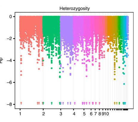
In this paper, we looked at the rest of the genome of the same chickens — you didn’t think we sequenced the whole thing just to look at the mitochondrion plus a subset of markers, did you? We turn to population genomics, and a family of methods called selective sweep mapping, to search for regions of their genome that show signs of being affected by natural selection. This lets us: 1) draw pretty rainbow plots such as  this one …

kauai2_fig1a

(Figure 1a from the paper in question, Johnsson & al 2016. cc:by The chromosomes have been laid out on the horizontal axis with different colours, and split into windows of 40 kb. Each dot represents the heterozygosity of that windows. For all the details, see the paper.)

… 2) highlight a regions of the genome that may have been selected during feralisation on Kauai (these are the icicles in the graph, highligthed by arrows); 3) conclude that the regions that look like they’ve been selected in feralisation overlap very little with the ones that look like they’ve been selected in chicken domestication. Hence the title.

That was the main result, but of course we also look at what genes are highlighted. Mostly we have no idea how they may contribute to feralisation, but a couple of regions overlap with those that we’ve previously found in genetic mapping of comb size and egg laying in our wild-by-domestic intercross. We also compare the potentially selected regions to domestic chicken sequences.

Last year, Ewen Callaway visited Dominic Wright, Eben Gering and Rie Henriksen on the last fieldtrip to Kauai. The article, When chickens go wild, was published in Nature News in January, and it explains a lot of the ideas nicely. This paper was submitted by then, so the samples they gathered on that trip do not feature in it. But, spoiler alert: there is more to come. (I don’t know what role I personally will play, but that is less important.)

As you may have guessed if you looked at the author list, this was a collaboration between quite a lot of people in Linköping, Michigan, London, and Victoria. Thanks to all involved! This was great fun, and for those of you who like this sort of thing, I hope the paper will be an interesting read.

Literature

M. Johnsson, E. Gering, P. Willis, S. Lopez, L. Van Dorp, G. Hellenthal, R. Henriksen, U. Friberg & D. Wright. (2016) Feralisation targets different genomic loci to domestication in the chicken. Nature Communications. doi:10.1038/ncomms12950

R in genomics @ SciLifeLab, Solna

Dear diary,

I went to the Stockholm R useR group meetup on R in genomics at the Stockholm node of SciLifeLab. It was nice. If I had worked a bit closer I would attend meetups all the time. I even got to be pretentious with my notebook while waiting for the train.

blog_pretentious

The speakers were:

Jakub Orzechowski Westholm on R and genomics in general. He demonstrated genome browser-style tracks with Gviz, some GenomicRanges, and a couple of common plots of gene expression data. I have been on the fence about what package I should use for drawing genes and variants along the genome. I should play with Gviz.

Daniel Klevebring on clinical sequencing and how he uses R (not that much) in sequencing pipelines aimed at targeting the right therapy to patients based on the mutations in their cancer cells. He mentioned some getopt snippets for getting R to play nicely on the command line, which is something I should definitely try more!

Finally, Arvind Singh Mer on predictive modelling for clinical genomics (like the abovementioned ClinSeq data). He showed the caret package for machine learning, with an elastic net regression.

I don’t know the rest of the audience, so maybe the choice to gear talks towards the non-bio* person was spot on, but that made things a bit less interesting for me. For instance, in Jakub’s talk about gene expression, I would’ve preferred more about the messy stuff: how to make that nice gene-by-sample matrix in the first place, and if R can be of any help in that process; also, in the other end, what models one would use after that first pass of visualisation. But this isn’t a criticism of the presenters — time and complexity constraints apply. (If I was asked to present how I use R any demos would be toy analyses of clean datasets. That is the way these things go.)

We also heard repeated praise for and recommendations of the hadleyverse and data.table. I’m not a data.tabler myself, but I probably should be. And I completely agree about the value of dplyr — there’s this one analysis where a couple of lines with dplyr changed it from ”argh, do I have to rewrite this in C?” to being workable. I think we also saw all the three plotting systems: base graphics, ggplot2 and lattice in action.

From my halftime seminar

A couple of weeks ago I presented my halftime seminar at IFM Biology, Linköping university. The halftime at our department isn’t a particularly dramatic event, but it means that after you’ve been going for two and a half years (since a typical Swedish PhD programme is four years plus 20% teaching to a total of five years), you get to talk about what you’ve been up to and discuss it with an invited opponent. I talked about combining genetic mapping and gene expression to search for quantitative trait genes for chicken domestication traits, and the work done so far particularly with relative comb mass. To give my esteemed readers an overview of what my project is about, here come a few of my slides about the mapping work — it is described in detail in Johnsson & al (2012). Yes, it does feel very good to write that — shout-outs to all the coauthors! This is part what I said on the seminar, part digression more suited for the blog format. Enjoy!

Slide04(Photo: Dominic Wright)

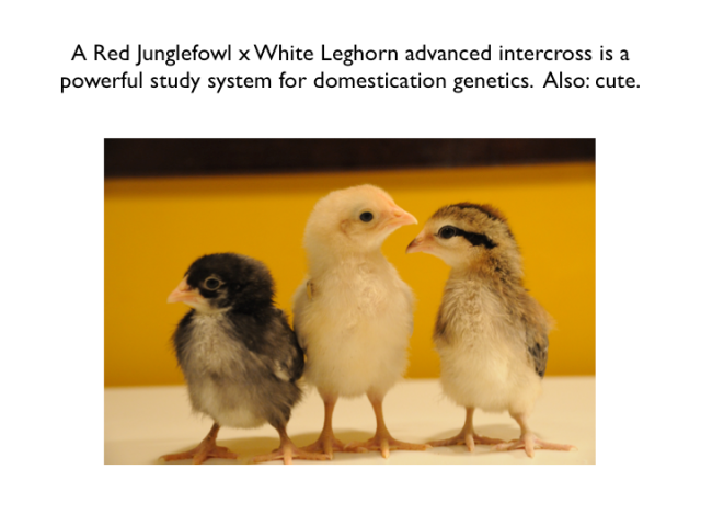
The common theme of my PhD project is genetic mapping and genetical genomics in an experimental intercross of wild and domestic chickens. The photo shows some of them as chicks. Since plumage colour is one of the things that segregate in this cross, their feathers actually make a very nice illustration of what is going on. We’re interested in traits that differ between wild and domestic chickens, so we use a cross based on a Red Jungefowl male and three domestic White Leghorn females. Their offspring have been mated with each other for several generations, giving rise to what is called an advanced intercross line. Genetic variants that cause differences between White Leghorn and Red Jungefowl chickens will segregate among the birds of the cross, and are mixed by recombination at meiosis. Some of the birds have the Red Junglefowl variant and some have the White Leghorn variant at a given part of their genome. By measuring traits that vary in the cross, and genotyping the birds for a map of genetic markers, we can find chromosomal chunks that are associated with particular traits, i.e. regions of the genome where we’re reasonably confident harbour a variant affecting the trait. These chromosomal chunks tend to be rather large, though, and contain several genes. My job is to use gene expression measurements from the cross to help zero in on the right genes.

The post continues below the fold! Fortsätt läsa