A few months ago I saw this nice figure from Amy Williams of the number of DNA segments that are expected to be shared between relatives. I thought it would be fun to simulate segment sharing with AlphaSimR.

Because DNA comes in chromosomes that don’t break up and recombine that much, the shared DNA between relatives tends to come in long chunks — segments that are identical by descent. The distribution of segment lengths can sometimes be used to tell apart relationships that would otherwise give the same average (e.g., Yengo et al. 2019, Qiao et al. 2021).

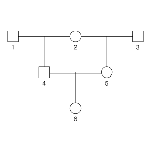
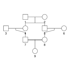
But let’s not do anything sophisticated. Instead, we take three very simple pedigrees — anyone who’s taken introductory genetics will recognize these ones — and look at relationships between full-sibs, half-sibs and cousins. We’ll also look at the inbred offspring of matings between full-sibs, half-sibs and cousins to see that the proportion that they share between their two copies of the genome lines up with the expected inbreeding.

There won’t be any direct comparison to the values that Williams’ simulation, because it simulated more distant relationships than this, starting with cousins and then moving further away. This is probably more interesting, especially for human genealogical genetics.

The code is on GitHub if you wants to follow along.

The pedigrees

Here are the three pedigrees, drawn with the kinship2 package:

A pedigree, here, is really a table of individuals, where each column tells us their identifier, their parents, and optionally their sex, like this:

id, mother, father, sex
1, NA, NA, M
2, NA, NA, F
3, NA, NA, M
4, 2, 1, F
5, 2, 1, M
6, NA, NA, F
7, 4, 3, M
8, 6, 5, F
9, 8, 7, F

We can use GeneticsPed to check the relatedness and inbreeding if we don’t trust that I’ve entered the pedigrees right.

library(GeneticsPed)
library(purrr)
library(readr)

ped_fullsib <- read_csv("pedigrees/inbreeding_fullsib.txt")
ped_halfsib <- read_csv("pedigrees/inbreeding_halfsib.txt")
ped_cousin <- read_csv("pedigrees/inbreeding_cousin.txt")

inbreeding_ped <- function(ped) {

    inbreeding(Pedigree(ped))

}

print(map(list(ped_fullsib, ped_halfsib, ped_cousin), inbreeding_ped))

[[1]]
   1    2    3    4    5 
0.00 0.00 0.00 0.00 0.25 

[[2]]
    1     2     3     4     5     6 
0.000 0.000 0.000 0.000 0.000 0.125 

[[3]]
     1      2      3      4      5      6      7      8      9 
0.0000 0.0000 0.0000 0.0000 0.0000 0.0000 0.0000 0.0000 0.0625

Comparing haplotypes

We need some functions to compare haplotypes and individuals:

library(AlphaSimR)
library(dplyr)
library(purrr)
library(tibble)

## Find shared segments between two haplotypes expressed as vectors
## map is a vector of marker positions

compare_haplotypes <- function(h1, h2, map) {
    sharing <- h1 == h2

    runs <- rle(sharing)
    end <- cumsum(runs$lengths)
    start <- c(1, end[-length(end)] + 1)

    segments <- tibble(start = start,
                       end = end,
                       start_pos = map[start],
                       end_pos = map[end],
                       segment_length = end_pos - start_pos,
                       value = runs$values)

    segments[segments$value,]
}

We will have haplotypes of the variants that go together on a chromosome, and we want to find segments that are shared between them. We do this with a logical vector that tests each variant for equality, and then use the rle to turn this into run-length encoding. We extract the start and end position of the runs and then keep only the runs of equality.

Building on that function, we want to find the shared segments on a chromosome between two individuals. That is, we make all the pairwise comparisons between the haplotypes they carry and combine them.

## Find shared segments between two individuals (expressed as
## matrices of haplotypes) for one chromosome

compare_individuals_chr <- function(ind1, ind2, map) {

    h1_1 <- as.vector(ind1[1,])
    h1_2 <- as.vector(ind1[2,])

    h2_1 <- as.vector(ind2[1,])
    h2_2 <- as.vector(ind2[2,])

    sharing1 <- compare_haplotypes(h1_1, h2_1, map)
    sharing2 <- compare_haplotypes(h1_1, h2_2, map)
    sharing3 <- compare_haplotypes(h1_2, h2_1, map)
    sharing4 <- compare_haplotypes(h1_2, h2_2, map)

    bind_rows(sharing1, sharing2, sharing3, sharing4)
}

Finally, we use that function to compare individuals along all the chromosomes.

This function takes in a population and simulation parameter object from AlphaSimR, and two target individuals to be compared.

We use AlphaSimR‘s pullIbdHaplo function to extract tracked founder haplotypes (see below) and then loop over chromosomes to apply the above comparison functions.

## Find shared segments between two target individuals in a
## population

compare_individuals <- function(pop,
                                target_individuals,
                                simparam) {

    n_chr <- simparam$nChr

    ind1_ix <- paste(target_individuals[1], c("_1", "_2"), sep = "")
    ind2_ix <- paste(target_individuals[2], c("_1", "_2"), sep = "")

    ibd <- pullIbdHaplo(pop,
                        simParam = simparam)

    map <- simparam$genMap
    loci_per_chr <- map_dbl(map, length)

    chr_ends <- cumsum(loci_per_chr)
    chr_starts <- c(1, chr_ends[-n_chr] + 1)

    results <- vector(mode = "list",
                      length = n_chr)

    for (chr_ix in 1:n_chr) {

        ind1 <- ibd[ind1_ix, chr_starts[chr_ix]:chr_ends[chr_ix]]
        ind2 <- ibd[ind2_ix, chr_starts[chr_ix]:chr_ends[chr_ix]]

        results[[chr_ix]] <- compare_individuals_chr(ind1, ind2, map[[chr_ix]])
        results[[chr_ix]]$chr <- chr_ix
    }

    bind_rows(results)
}

(You might think it would be more elegant, when looping over chromosomes, to pull out the identity-by-descent data for each chromosome at a time. This won’t work on version 1.0.4 though, because of a problem with pullIbdHaplo which has been fixed in the development version.)

We use an analogous function to compare the haplotypes carried by one individual. See the details on GitHub if you’re interested.

Building the simulation

We are ready to run our simulation: This code creates a few founder individuals that will initiate the pedigree, and sets up a basic simulation. The key simulation parameter is to set setTrackRec(TRUE) to turn on tracking of recombinations and founder haplotypes.

source("R/simulation_functions.R")

## Set up simulation

founders <- runMacs(nInd = 10,
                    nChr = 25)

simparam <- SimParam$new(founders)

simparam$setTrackRec(TRUE)

founderpop <- newPop(founders,
                     simParam = simparam)

To simulate a pedigree, we use pedigreeCross, a built-in function to simulate a given pedigree, and then apply our comparison functions to the resulting simulated population.

## Run the simulation for a pedigree one replicate

simulate_pedigree <- function(ped,
                              target_individuals,
                              focal_individual,
                              founderpop,
                              simparam) {
    pop <- pedigreeCross(founderPop = founderpop,
                         id = ped$id,
                         mother = ped$mother,
                         father = ped$father,
                         simParam = simparam)
    shared_parents <- compare_individuals(pop,
                                          target_individuals,
                                          simparam)
    shared_inbred <- compare_self(pop,
                                  focal_individual,
                                  simparam)
    list(population = pop,
         shared_segments_parents = shared_parents,
         shared_segments_self_inbred = shared_inbred)
}

Results

First we can check how large proportion of the genome of our inbred individuals is shared between their two haplotypes, averaged over 100 replicates. That is, how much of the genome is homozygous identical by descent — what is their genomic inbreeding? It lines up with the expectation form pedigree: 0.25 for the half-sib pedigree, close to 0.125 for the full-sib pedigree and close to 0.0625 for the cousin pedigree. The proportion shared by the parents is, as it should, about double that.

      case inbred_self_sharing parent_sharing
  full-sib        0.25 (0.052)    0.5 (0.041)
  half-sib        0.13 (0.038)   0.25 (0.029)
    cousin       0.064 (0.027)   0.13 (0.022)

Table of the mean proportion of genome shared between the two genome copies in inbred individuals and between their parents. Standard deviations in parentheses.

This is a nice consistency check, but not really what we wanted. The point of explicitly simulating chromosomes and recombinations is to look at segments, not just total sharing.

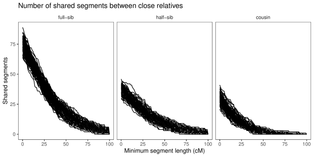
With a little counting and summarisation, we can plot the distributions of segment lengths. The horizontal axis is the length of the segments expressed in centimorgan. The vertical axis is the number of shared
segments of this length or longer. Each line is a replicate.

If we look at the summaries (table below), full-sibs share on average 74 segments greater than 1 cM in length, half-sibs 37, and cousins 29.

In real data, short segments might be harder to detect, but because we’re using simulated fake data, we don’t have to worry about phasing errors or false positive sharing.

If we look only at long segments (> 20 cM), full-sibs share on average 46 segments, half-sibs 23, and cousins 13. (Also, similar to Williams’ simulations, none of the cousins simulated here had less than five long segments shared.)

  case     `1 cM`   `10 cM`  `20 cM`  `30 cM`  `40 cM`  
  full-sib 74 (5.2) 60 (4.2) 46 (3.6) 34 (4)   24 (3.8) 
  half-sib 37 (3.4) 30 (3.1) 23 (3.3) 17 (2.8) 13 (2.6) 
  cousin   29 (3.8) 20 (3.3) 13 (3.2) 7.6 (2)  4.3 (1.8)

Table of the mean number of shared segments of different minimum length. Standard deviations in parentheses.

We an also look at the average length of the segments shared, and note that while full-sibs and half-sibs differ in the number of segments, and total segment length shared (above), the length of individual segments is about the same:

  case     mean_length_sd
  full-sib 0.33 (0.032)  
  half-sib 0.34 (0.042)  
  cousin   0.21 (0.03)

Table of the mean length shared segments. Standard deviations in parentheses.

Limitations

Williams’ simulation, using the ped-sim tool, had a more detailed model of recombination in the human genome, with different interference parameters for each chromosome, sex-specific recombination and so on. In that way, it is much more realistic.
We’re not modelling any one genome in particular, but a very generic genome. Each chromosome is 100 cM long for example; one can imagine that a genome with many short chromosomes would give a different distribution. This can be changed, though; the chromosome size is the easiest, if we just pick a species.

Literature

Yengo, L., Wray, N. R., & Visscher, P. M. (2019). Extreme inbreeding in a European ancestry sample from the contemporary UK population. Nature communications, 10(1), 1-11.

Qiao, Y., Sannerud, J. G., Basu-Roy, S., Hayward, C., & Williams, A. L. (2021). Distinguishing pedigree relationships via multi-way identity by descent sharing and sex-specific genetic maps. The American Journal of Human Genetics, 108(1), 68-83.