In 2010, Poliseno & co published some results on the regulation of a gene by a transcript from a pseudogene. Now, Kerwin & co have published a replication study, the protocol for which came out in 2015 (Khan et al). An editor summarises it like this in an accompanying commentary (Calin 2020):

The partial success of a study to reproduce experiments that linked pseudogenes and cancer proves that understanding RNA networks is more complicated than expected.

I guess he means ”partial success” in the sense that they partially succeeded in performing the replication experiments they wanted. These experiments did not reproduce the gene regulation results from 2010.

Seen from the outside — I have no insight in what is going on here or who the people involved are — something is not working here. If it takes five years from paper to replication effort, and then another five years to replication study accompanied by an editorial commentary that subtly undermines it, we can’t expect replication studies to update the literature, can we?

Communication

What’s the moral of the story, according to Calin?

What are the take-home messages from this Replication Study? One is the importance of fruitful communication between the laboratory that did the initial experiments and the lab trying to repeat them. The lack of such communication – which should extend to the exchange of protocols and reagents – was the reason why the experiments involving microRNAs could not be reproduced. The original paper did not give catalogue numbers for these reagents, so the wrong microRNA reagents were used in the Replication Study. The introduction of reporting standards at many journals means that this is less likely to be an issue for more recent papers.

There is something right and something wrong about this. On the one hand, talking to your colleagues in the field obviously makes life easier. We would like researchers to put all pertinent information in writing, and we would like there to be good communication channels in cases where the information turns out not to be what the reader needed. On the other hand, we don’t want science to be esoteric. We would like experiments to be reproducible without the special artifact or secret sauce. If nothing else, because the people’s time and willingness to provide tech support for their old papers might be limited. Of course, this is hard, in a world where the reproducibility of an experiment might depend on the length of digestion (Hines et al 2014) or that little plastic thingamajig you need for the washing step.

Another take-home message is that it is finally time for the research community to make raw data obtained with quantitative real-time PCR openly available for papers that rely on such data. This would be of great benefit to any group exploring the expression of the same gene/pseudogene/non-coding RNA in the same cell line or tissue type.

This is true. You know how doctored, or just poor, Western blots are a notorious issue in the literature? I don’t think that’s because Western blot as a technique is exceptionally bad, but because there is a culture of showing the raw data (the gel), so people can notice problems. However, even if I’m all for showing real-time PCR amplification curves (as well as melting curves, standard curves, and the actual batch and plate information from the runs), I doubt that it’s going to be possible to trouble-shoot PCR retrospectively from those curves. Maybe sometimes one would be able to spot a PCR that looks iffy, but beyond that, I’m not sure what we would learn. PCR issues are likely to have to do with subtle things like primer design, reaction conditions and handling that can only really be tackled in the lab.

The world is messy, alright

Both the commentary and the replication study (Kerwin et al 2020) are cautious when presenting their results. I think it reads as if the authors themselves either don’t truly believe their failure to replicate or are bending over backwards to acknowledge everything that could have gone wrong.

The original study reported that overexpression of PTEN 3’UTR increased PTENP1 levels in DU145 cells (Figure 4A), whereas the Replication Study reports that it does not. …

However, the original study and the Replication Study both found that overexpression of PTEN 3’UTR led to a statistically significant decrease in the proliferation of DU145 cells compared to controls.

In the original study Poliseno et al. reported that two microRNAs – miR-19b and miR-20a – suppress the transcription of both PTEN and PTENP1 in DU145 prostate cancer cells (Figure 1D), and that the depletion of PTEN or PTENP1 led to a statistically significant reduction in the corresponding pseudogene or gene (Figure 2G). Neither of these effects were seen in the Replication Study. There are many possible explanations for this. For example, although both studies used DU145 prostate cancer cells, they did not come from the same batch, so there could be significant genetic differences between them: see Andor et al. (2020) for more on cell lines acquiring mutations during cell cultures. Furthermore, one of the techniques used in both studies – quantitative real-time PCR – depends strongly on the reagents and operating procedures used in the experiments. Indeed, there are no widely accepted standard operating procedures for this technique, despite over a decade of efforts to establish such procedures (Willems et al., 2008; Schwarzenbach et al., 2015).

That is both commentary and replication study seem to subscribe to a view of the world where biology is so rich and complex that both might be right, conditional on unobserved moderating variables. This is true, but it throws us into a discussion of generalisability. If a result only holds in some genotypes of DU145 prostate cancer cells, which might very well be the case, does it generalise enough to be useful for cancer research?

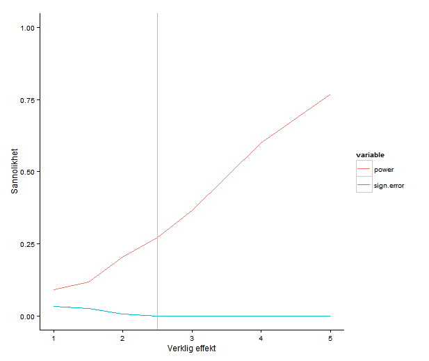
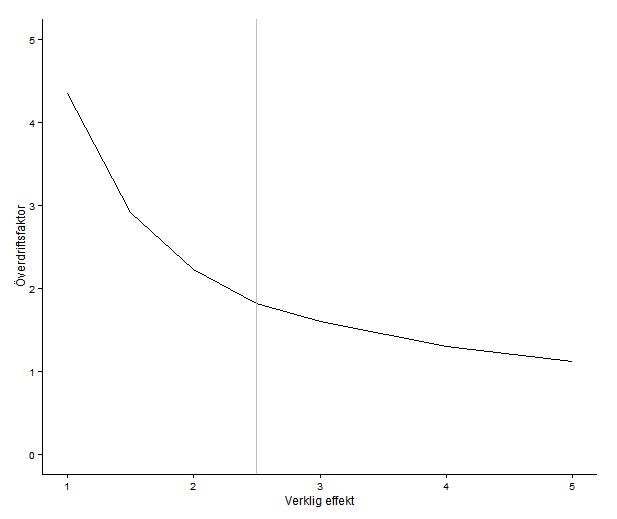
Power underwhelming

There is another possible view of the world, though … Indeed, biology rich and complicated, but in the absence of accurate estimates, we don’t know which of all these potential moderating variables actually do anything. First order, before we start imagining scenarios that might explain the discrepancy, is to get a really good estimate of it. How do we do that? It’s hard, but how about starting with a cell size greater than N = 5?

The registered report contains power calculations, which is commendable. As far as I can see, it does not describe how they arrived at the assumed effect sizes. Power estimates for a study design depend on the assumed effect sizes. Small studies tend to exaggerate effect sizes (because, if an estimate is small the difference can’t be significant). This means that taking the estimates as staring effect sizes might leave you with a design that is still unable to detect a true effect of reasonable size.

I don’t know what effect sizes one should expect in these kinds of experiments, but my intuition would be that even if you think that you can get good power with a handful of samples per cell, can’t you please run a couple more? We are all limited by resources and time, but if you’re running something like a qPCR, the cost per sample must be much smaller than the cost for doing one run of the experiment in the first place. It’s really not as simple as adding one row on a plate, but almost.

Literature

Calin, George A. ”Reproducibility in Cancer Biology: Pseudogenes, RNAs and new reproducibility norms.” eLife 9 (2020): e56397.

Hines, William C., et al. ”Sorting out the FACS: a devil in the details.” Cell reports 6.5 (2014): 779-781.

Kerwin, John, and Israr Khan. ”Replication Study: A coding-independent function of gene and pseudogene mRNAs regulates tumour biology.” eLife 9 (2020): e51019.

Khan, Israr, et al. ”Registered report: a coding-independent function of gene and pseudogene mRNAs regulates tumour biology.” Elife 4 (2015): e08245.

Poliseno, Laura, et al. ”A coding-independent function of gene and pseudogene mRNAs regulates tumour biology.” Nature 465.7301 (2010): 1033-1038.