Paper: ”Genetic variation in recombination rate in the pig”

Our paper on genetic variation in recombination in the pig just came out the other week. I posted about it already when it was a preprint, but we dug a little deeper into some of the results in response to peer review, so let us have a look at it again.

Summary

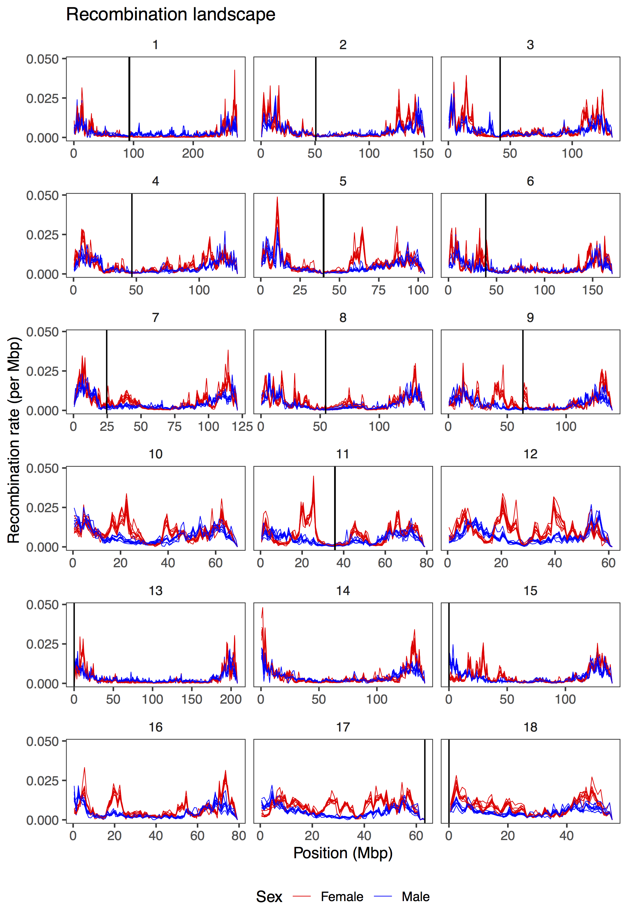
Recombination between chromosomes during meiosis leads to shuffling of genetic material between chromosomes, creating new combinations of alleles. Recombination rate varies, though, between parts of the genome, between sexes, and between individuals. Illustrating that, here is a figure from the paper showing how recombination rate varies along the chromosomes of the pig genome. Female recombination rate is higher than male recombination rate on most chromosomes, and in particular in regions of higher recombination rate in the middle of certain chromosomes.

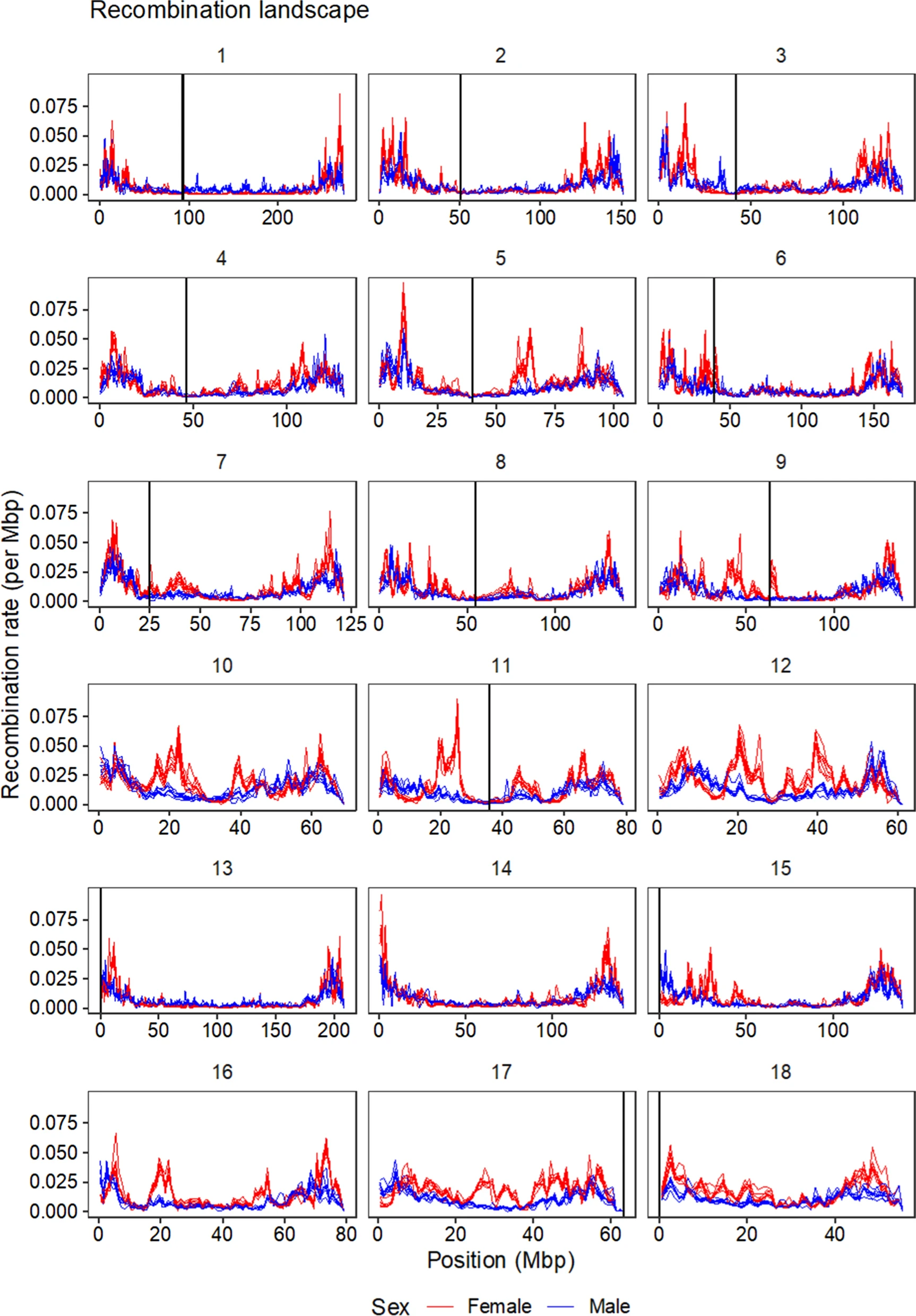
Fig 2 from the paper: average recombination rate in 1 Mbp windows along the pig genome. Each line is a population, coloured by sexes.

In several other vertebrates, part of that individual variation in recombination rate (in the gametes passed on by that individual) is genetic, and associated with regions close to known meiosis-genes. It turns out that this is the case in the pig too.

In this paper, we estimated recombination rates in nine genotyped pedigree populations of pigs, and used that to perform genome-wide association studies of recombination rate. The heritability of autosomal recombination rate was around 0.07 in females, 0.05 in males.

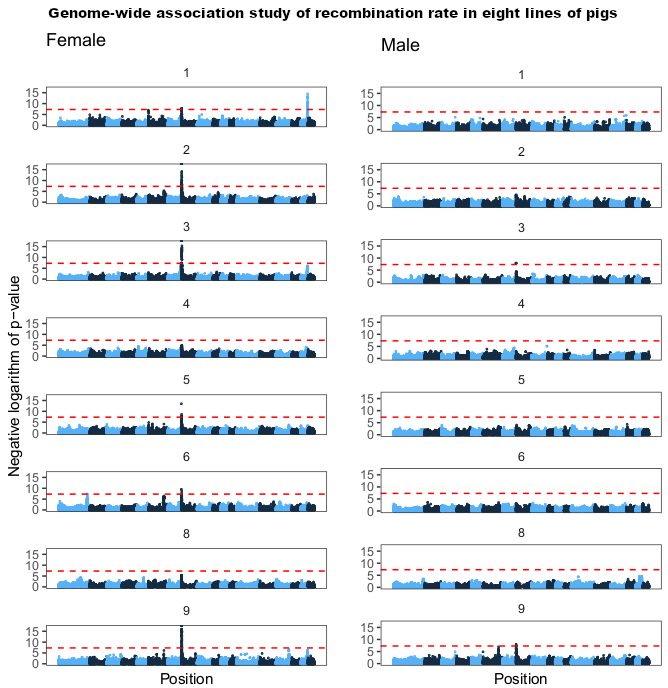
The major genome-wide association hit on chromosome 8, well known from other mammals, overlapped the RNF212 gene in most populations in females, and to a lesser extent in males.

Fig 6 from the paper, showing genome-wide association results for eight of the populations (one had too few individuals with recombination rate estimates after filtering for GWAS). The x-axis is position in the genome, and the y-axis is the negative logarithm of the p-value from a linear mixed model with repeated measures.

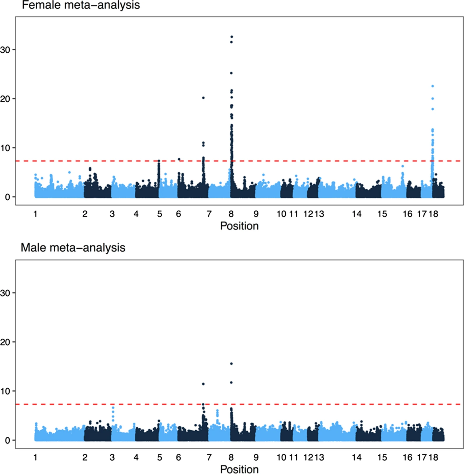
One of the things we added after the preprint is a meta-analysis of genome-wide association over all the populations (separated by sex). In total, there were six associated regions, five of which are close to known recombination genes: RNF212, SHOC1, SYCP2, MSH4 and HFM1. In particular, several of the candidates are genes involved in whether a double strand break resolves as a crossover or non-crossover. However, we do not have the genomic resolution to know whether these are actually the causative genes; there are significant markers overlapping many genes, and the candidate genes are not always the closest gene.

How well does the recombination landscape agree with previous maps?

The recombination landscapes accord pretty well with Tortereau et al.’s (2012) maps. We find a similar sex difference, with higher recombination in females on all autosomes except chromosome 1 and 13, and a stronger association with GC content in females. However, our recombination rates tend to be higher, possibly due to some overestimation. Different populations, where recombinations are estimated independently, also have similar recombination landscapes.

But it doesn’t agree so well with Lozada-Soto et al. (2021), does it?

No, that is true. Between preprint and finished version, Lozada-Soto et al. (2021) published a genome-wide association study of recombination rate in the pig. They found heritabilities of recombination rate of a similar magnitude as we did, but their genome-wide association results are completely different. We did not find the hits that they found, and they did not find the hits we found, or any previously known candidate genes for recombination. To be honest, I don’t have a good explanation for these differences.

How about recombination hotspots and PRDM9?

At a very fine scale, most recombination tends to occur in hotspots of around a few kilobasepairs. As this study used pedigrees and SNP chips with much coarser density than this, we cannot say much about the fine-scale recombination landscape. We work, at the finest, with windows of 1 Mbp. However, as the pig appears to have a working and rapidly evolving PRDM9 gene (encoding a protein that is responsible for recombination hotspot targeting), the pig probably has a PRDM9-based landscape of hotspots just like humans and mice (Baker et al. 2019).

Tortereau et al. (2012) found a positive correlation between counts of the PRDM9 DNA-binding motif and recombination rate, which is biologically plausible, as more PRDM9 motifs should mean more hotspots. So, we estimated this correlation for comparison, but found only a very weak relationship — this is one point where our results are inconsistent with previous maps. This might be because of changes in improved pig genome assembly we use, or it might be an indication that we have worse genomic resolution due to the genotype imputation involved in our estimation. However, one probably shouldn’t expect to find strong relationships between a process at the kilobasepair-scale when using windows of 1 Mbp in the first place.

Can one breed for increased recombination to improve genetic gain?

Not really. Because recombination breaks up linkage disequlibrium between causative variants, higher recombination rate could reveal genetic variation for selection and improve genetic gain. However, previous studies suggest that recombination rate needs to increase quite a lot (two-fold or more) to substantially improve breeding (Battagin et al. 2016). We made some back of the envelope quantitative genetic calculations on the response to selection for recombination, and it would be much smaller than that.

Literature

Johnsson M*, Whalen A*, Ros-Freixedes R, Gorjanc G, Chen C-Y, Herring WO, de Koning D-J, Hickey JM. (2021) Genetics variation in recombination rate in the pig. Genetics Selection Evolution (* equal contribution)

Tortereau, F., Servin, B., Frantz, L., Megens, H. J., Milan, D., Rohrer, G., … & Groenen, M. A. (2012). A high density recombination map of the pig reveals a correlation between sex-specific recombination and GC content. BMC genomics, 13(1), 1-12.

Lozada‐Soto, E. A., Maltecca, C., Wackel, H., Flowers, W., Gray, K., He, Y., … & Tiezzi, F. (2021). Evidence for recombination variability in purebred swine populations. Journal of Animal Breeding and Genetics, 138(2), 259-273.

Baker, Z., Schumer, M., Haba, Y., Bashkirova, L., Holland, C., Rosenthal, G. G., & Przeworski, M. (2017). Repeated losses of PRDM9-directed recombination despite the conservation of PRDM9 across vertebrates. Elife, 6, e24133.

Battagin, M., Gorjanc, G., Faux, A. M., Johnston, S. E., & Hickey, J. M. (2016). Effect of manipulating recombination rates on response to selection in livestock breeding programs. Genetics Selection Evolution, 48(1), 1-12.

Preprint: ”Genetics of tibia bone properties of crossbred commercial laying hens in different housing systems”

We have a new preprint posted to Biorxiv looking into the genetic basis of bone strength and other bone properties in crossbred laying hens in two different housing environments (furnished cages and floor pens).

Here are the citation and abstract:

Martin Johnsson, Helena Wall, Fernando A Lopes Pinto, Robert H. Fleming, Heather A. McCormack, Cristina Benavides-Reyes, Nazaret Dominguez-Gasca, Estefania Sanchez-Rodriguez, Ian C. Dunn, Alejandro B. Rodriguez-Navarro, Andreas Kindmark, Dirk-Jan de Koning (2021) Genetics of tibia bone properties of crossbred commercial laying hens in different housing systems. bioRxiv 2021.06.21.449243

Osteoporosis and bone fractures are a severe problem for the welfare of laying hens, with genetics and environment, such as housing system, each making substantial contributions to bone strength. In this work, we performed genetic analyses of bone strength, bone mineral density and bone composition, as well as body weight, in 860 commercial crossbred laying hens from two different companies, kept in either furnished cages or floor pens. We compared bone traits between housing systems and crossbreds, and performed a genome-wide association study of bone properties and body weight.

As expected, the two housing systems produced a large difference in bone strength, with layers housed in floor pens having stronger bones. These differences were accompanied by differences in bone geometry, mineralisation and chemical composition. Genome-scans either combining or independently analysing the two housing systems revealed no genome-wide significant loci for bone breaking strength. We detected three loci for body weight that were shared between the housing systems on chromosomes 4, 6 and 27 (either genome-wide significant or suggestive when the housing systems were analysed individually) and these coincide with associations for bone length.

In summary, we found substantial differences in bone strength, content and composition between hens kept in floor pens and furnished cages that could be attributed to greater physical activity in pen housing. We found little evidence for large-effect loci for bone strength in commercial crossbred hens, consistent with a highly polygenic architecture for bone strength in the production environment. The lack of consistent genetic associations between housing systems in combination with the differences in bone phenotypes support gene-by-environment interactions with housing system.

The background is that bone quality is a serious problem for laying hens; that housing systems that allow for more movement are known to lead to stronger bones; and that previous work on the genetics of bone parameters comes mostly from pure lines or from experimental intercrosses between divergent lines. Here, we study commercial crossbred laying hens from two different companies.

Being housed in a floor pen, where there is more opportunity for physical activity, or in a furnished cage makes a big difference to bone breaking strength. For comparison, we also show body weight, which is not much different between the housing environments. This difference was accompanied by differences in bone composition (see details in the paper).

And here are the Manhattan plots from genome-wide association: bone strength shows no major loci, as opposed to body weight, which has strong associations that are shared between the housing systems.

And if we compare the genome-wide associations, marker for marker, between the housing systems, there is nothing in common between the suggestive associations for bone strength. (Body weight below for comparison.)

This includes not detecting major loci for bone strength that have been found in pure lines of chickens. We think this is due to gene-by-environment interactions with housing (i.e. physical activity). This might be a complication for genomic selection for bone quality, as selection might need to be targeted to different housing systems.

Finally, the three strong association for body weight shown above overlap previously detected loci on chromosomes 4, 6, and 27. We do not have the genomic resolution to nominate candidate genes with any confidence, but the chromosome 4 locus overlaps both the CCKAR gene, which is a strong candidate for growth and body mass in the chicken and the LCORL/NCAPG locus, which has been associated with body size in several species. These regions (plus a fourth one) are also associated with bone length:

Journal club of one: ”Genome-wide enhancer maps link risk variants to disease genes”

(Here is a a paper from a recent journal club.)

Nasser et al. (2021) present a way to prioritise potential noncoding causative variants. This is part of solving the fine mapping problem, i.e. how to find the underlying causative variants from genetic mapping studies. They do it by connecting regulatory elements to genes and overlapping those regulatory elements with variants from statistical fine-mapping. Intuitively, it might not seem like connecting regulatory elements to genes should be that hard, but it is a tricky problem. Enhancers — because that is the regulatory element most of this is about; silencers and insulators get less attention — do not carry any sequence that tells us what gene they will act on. Instead, this needs to be measured or predicted somehow. These authors go the measurement route, combining chromatin sequencing with chromosome conformation capture.

This figure from the supplementary materials show what the method is about:

Additional figure 1 from Nasser et al. (2021) showing an overview of the workflow and an example of two sets of candidate variants derived from-fine mapping, each with variants that overlap enhancers connected to IL10.

They use chromatin sequence data (such as ATAC-seq, histone ChIP-seq or DNAse-seq) in combination with HiC chromosome conformation capture data to identify enhancers and connect them to genes (this was developed earlier in Fulco et al. 2019). The ”activity-by-contact model” means to multiply the contact frequency (from HiC) between promoter and enhancer with the enhancer activity (read counts from chromatin sequencing), standardised by the total contact–activity product with all elements within a window. Fulco et al. (2019) previously found that this conceptually simple model did well at connecting enhancers to genes (as evaluated with a CRISPR inhibition assay called CRISPRi-FlowFISH, which we’re not going into now, but it’s pretty ingenious).

In order to use this for fine-mapping, they calculated activity-by-contact maps for every gene combined with every open chromatin element within 5 Mbp for 131 samples from ENCODE and other sources. The HiC data were averaged of contacts in ten cell types, transformed to be follow a power-law distribution. That is, they did not do the HiC analysis per cell type, but use the same average HiC contact matrix combined with chromatin data from different cell types. Thus, the specificity comes from the promoters and enhancers that are called as active in each sample — I assume this is because the HiC data comes from a different (and smaller) set of cell types than the chromatin sequencing. Element–gene pairs that reached above a threshold were considered connected, for a total of about six million connections, involving 23,000 genes and 270,000 enhancers. On average, a gene had 2.8 enhancers and an enhancer connected to 2.7 genes.

They picked putative causative variants by overlapping the variant sets with these activity-by-contact maps and selecting the highest scoring enhancer gene pair.They used fine-mapping results from multiple previous studies. These variants were estimated with different methods, but they are all some flavour of fine-mapping by variable selection. Statistical fine mapping estimate sets of variants, called credible sets, that have high posterior probability of being the causative variant. They included only completely noncoding credible sets, i.e. those that did not include a coding sequence or splice variant. They applied this to 72 traits in humans, generating predictions for ~ 5000 noncoding credible sets of variants.

Did it work?

Variants for fine-mapping were enriched in connected enhancers more than in open chromatin in general, in cell types that are relevant to the traits. In particular, inflammatory bowel disease variants were enriched in enhancers in 65 samples, including immune cell types and gut cells. The strongest enrichment was in activated dendritic cells.

They used a set of genes previously known to be involved in inflammatory bowel disease, assuming that they were the true causative genes for their respective noncoding credible sets, and then compared their activity-by-contact based prioritisation of the causative gene to simply picking the closest gene. Picking the closest gene was right in 30 out of 37 sets. Picking the gene with the highest activity-by-contact score was right in 17 cases out of 18 sets that overlapped an activity-by-contact enhancer. Thus, this method had higher precision but worse recall. They also tested a number of eQTL-based, enrichment and enhancer–gene mapping methods, that did worse.

What it tells us about causative variants

Most of the putative causative variants, picked based on maximising activity-by-contact, were close to the proposed gene (median 13 kbp) and most involved the closest gene (77%). They were often found their putative causative variants to be located in enhancers that were only active in a few cell- or tissue types (median 4), compared to the promoters of the target genes, that were active in a broader set (median 120). For example, in inflammatory bowel disease, there were several examples where the putatively causal enhancer was only active in a particular immune cell or a stimulated state of an immune cell.

My thoughts

What I like about this model is that it is so different to many of the integrative and machine learning methods we see in genomics. It uses two kinds of data, and relatively simple computations. There is no machine learning. There is no sequence evolution or conservation analysis. Instead, measure two relevant quantities, standardise and preprocess them a bit, and then multiply them together.

If the success of the activity-by-contact model for prioritising causal enhancers generalises beyond the 18 causative genes investigated in the original paper, this is an argument for simple biology-based heuristics over machine learning models. It also suggest that, in the absence of contact data, one might do well by prioritising variant in enhancers that are highly active in relevant cell types, and picking the closest gene as the proposed causative gene.

However, the dataset needs to cover the relevant cell types, and possibly cells that are in the relevant stimulated states, meaning that it provides a motivation for rich conditional atlas-style datasets of chromatin and chromosome conformation.

I am, personally, a little bit sad that expression QTL methods seem to doing poorly. On the other hand, it makes some sense that eQTL might not have the genomic resolution to connect enhancers to genes.

Finally, if the relatively simple activity-by-contact model or the ridiculously simple method of ”picking the closest gene” beats machine learning models using the same data types and more, it suggests that the machine learning methods might not be solving theright problem. After all, they are not trained directly to prioritise variants for complex traits — because there are too few known causative variants for complex traits.

Literature

Fulco, C. P., Nasser, J., Jones, T. R., Munson, G., Bergman, D. T., Subramanian, V., … & Engreitz, J. M. (2019). Activity-by-contact model of enhancer–promoter regulation from thousands of CRISPR perturbations. Nature genetics.

Nasser, J., Bergman, D. T., Fulco, C. P., Guckelberger, P., Doughty, B. R., Patwardhan, T. A., … & Engreitz, J. M. (2021). Genome-wide enhancer maps link risk variants to disease genes. Nature.

My talk at the ChickenStress Genomics and Bioinformatics Workshop

A few months ago I gave a talk at the ChickenStress Genomics and Bioinformatics Workshop about genetic mapping of traits and gene expression.

ChickenStress is a European training network of researchers who study stress in chickens, as you might expect. It brings together people who work with (according to the work package names) environmental factors, early life experiences and genetics. The network is centered on a group of projects by early stage researchers — by the way, I think that’s a really good way to describe the work of a PhD student — and organises activities like this workshop.

I was asked to talk about our work from my PhD on gene expression and behaviour in the chicken (Johnsson & al. 2018, Johnsson & al. 2016), concentrating on concepts and methods rather than results. If I have any recurring readers, they will already know that brief is exactly what I like to do. I talked about the basis of genetic mapping of traits and gene expression, what data one needs to do it, and gave a quick demo for a flavour of an analysis workflow (linear mixed model genome-wide association in GEMMA).

Here are slides, and the git repository of the demo:

Journal club of one: ”Eliciting priors and relaxing the single causal variant assumption in colocalisation analyses”

This paper (Wallace 2020) is about improvements to the colocalisation method for genome-wide association studies called coloc. If you have an association to trait 1 in a region, and another association with trait 2, coloc investigates whether they are caused by the same variant or not. I’ve never used coloc, but I’m interested because setting reasonable priors is related to getting reasonable parameters for genetic architecture.

The paper also looks at how coloc is used in the literature (with default settings, unsurprisingly), and extends coloc to relax the assumption of only one causal variant per region. In that way, it’s a solid example of thoughtfully updating a popular method.

(A note about style: This isn’t the clearest paper, for a few reasons. The structure of the introduction is indirect, talking a lot about Mendelian randomisation before concluding that coloc isn’t Mendelian randomisation. The paper also uses numbered hypotheses H1-H4 instead of spelling out what they mean … If you feel a little stupid reading it, it’s not just you.)

coloc is what we old QTL mappers call a pleiotropy versus linkage test. It tries to distinguish five scenarios: no association, trait 1 only, trait 2 only, both traits with linked variants, both traits with the same variant.

This paper deals with the priors: What is the prior probability of a causal association to trait 1 only p_1, trait 2 only p_2, or both traits p_{12} , and are the defaults good?

They reparametrise the priors so that it becomes possible to get some estimates from the literature. They work with the probability that a SNP is causally associated with each trait (which means adding the probabilities of association q_1 = p_1 + p_{12} ) … This means that you can look at single trait association data, and get an idea of the number of marginal associations, possibly dependent on allele frequency. The estimates from a gene expression dataset and a genome-wide association catalog work out to a prior around 10 ^ {-4} , which is the coloc default. So far so good.

How about p_{12} ?

If traits were independent, you could just multiply q_1 and q_2. But not all of the genome is functional. If you could straightforwardly define a functional proportion, you could just divide by it.

You could also look at the genetic correlation between traits. It makes sense that the overall genetic relationship between two traits should inform the prior that you see overlap at this particular locus. This gives a lower limit for p_{12} . Unfortunately, this still leaves us dependent on what kinds of traits we’re analysing. Perhaps, it’s not so surprising that there isn’t one prior that universally works for all kinds of pairs of trait:

Attempts to colocalise disease and eQTL signals have ranged from underwhelming to positive. One key difference between outcomes is the disease-specific relevance of the cell types considered, which is consistent with variable chromatin state enrichment in different GWAS according to cell type. For example, studies considering the overlap of open chromatin and GWAS signals have convincingly shown that tissue relevance varies by up to 10 fold, with pancreatic islets of greatest relevance for traits like insulin sensitivity and immune cells for immune-mediated diseases. This suggests that p_{12} should depend explicitly on the specific pair of traits under consideration, including cell type in the case of eQTL or chromatin mark studies. One avenue for future exploration is whether fold change in enrichment of open chromatin/GWAS signal overlap between cell types could be used to modulate p_{12} and select larger values for more a priori relevant tissues.

Literature

Wallace, Chris. ”Eliciting priors and relaxing the single causal variant assumption in colocalisation analyses.” PLoS Genetics 16.4 (2020): e1008720.

Preprint: ”Genetics of recombination rate variation in the pig”

We have a new preprint posted, showing that recombination rate in the pig is lowly heritable and associated with alleles at RNF212.

We developed a new method to estimate recombinations in 150,000 pigs, and used that to estimate heritability and perform genome-wide association studies in 23,000.

Here is the preprint:

Johnsson M*, Whalen A*, Ros-Freixedes R, Gorjanc G, Chen C-Y, Herring WO, de Koning D-J, Hickey JM. (2020) Genetics of recombination rate variation in the pig. BioRxiv preprint. https://doi.org/10.1101/2020.03.17.995969 (* equal contribution)

Here is the abstract:

Background In this paper, we estimated recombination rate variation within the genome and between individuals in the pig for 150,000 pigs across nine genotyped pedigrees. We used this to estimate the heritability of recombination and perform a genome-wide association study of recombination in the pig.

Results Our results confirmed known features of the pig recombination landscape, including differences in chromosome length, and marked sex differences. The recombination landscape was repeatable between lines, but at the same time, the lines also showed differences in average genome-wide recombination rate. The heritability of genome-wide recombination was low but non-zero (on average 0.07 for females and 0.05 for males). We found three genomic regions associated with recombination rate, one of them harbouring the RNF212 gene, previously associated with recombination rate in several other species.

Conclusion Our results from the pig agree with the picture of recombination rate variation in vertebrates, with low but nonzero heritability, and a major locus that is homologous to one detected in several other species. This work also highlights the utility of using large-scale livestock data to understand biological processes.

Interpreting genome scans, with wisdom

Eric Fauman is a scientist at Pfizer who also tweets out interpretations of genome-wide association scans.

Background: There is a GWASbot twitter account which posts Manhattan plots with links for various traits from the UK Biobank. The bot was made by the Genetic Epidemiology lab at the Finnish Institute for Molecular Medicine and Harvard. The source of the results is these genome scans (probably; it’s little bit opaque); the bot also links to heritability and genetic correlation databases. There is also an EnrichrBot that replies with enrichment of chromatin marks (Chen et al. 2013). Fauman’s comments on some of the genome scans on his Twitter account.

Here are a couple of recent ones:

And here is his list of these threads as a Google Document.

This makes me thing of three things, two good, and one bad.

1. The ephemeral nature of genome scans

Isn’t it great that we’re now at a stage where a genome scan can be something to be tweeted or put en masse in a database, instead of published one paper per scan with lots of boilerplate. The researchers behind the genome scans say as much in their 2017 blog post on the first release:

To further enhance the value of this resource, we have performed a basic association test on ~337,000 unrelated individuals of British ancestry for over 2,000 of the available phenotypes. We’re making these results available for browsing through several portals, including the Global Biobank Engine where they will appear soon. They are also available for download here.

We have decided not to write a scientific article for publication based on these analyses. Rather, we have described the data processing in a detailed blog post linked to the underlying code repositories. The decision to eschew scientific publication for the basic association analysis is rooted in our view that we will continue to work on and analyze these data and, as a result, writing a paper would not reflect the current state of the scientific work we are performing. Our goal here is to make these results available as quickly as possible, for any geneticist, biologist or curious citizen to explore. This is not to suggest that we will not write any papers on these data, but rather only write papers for those activities that involve novel method development or more complex analytic approaches. A univariate genome-wide association analysis is now a relatively well-established activity, and while the scale of this is a bit grander than before, that in and of itself is a relatively perfunctory activity. [emphasis mine] Simply put, let the data be free.

That being said, when starting to write this post, first I missed a paper. It was pretty frustrating to find a detailed description of the methods: after circling back and forth between the different pages that link to each other, I landed on the original methods post, which is informative, and written in a light conversational style. On the internet, one would fear that this links may rot and die eventually, and a paper would probably (but not necessarily …) be longer-lasting.

2. Everything is a genome scan, if you’re brave enough

Another thing that the GWAS bot drives home is that you can map anything that you can measure. The results are not always straightforward. On the other hand, even if the trait in question seems a bit silly, the results are not necessarily nonsense either.

There is a risk, for geneticists and non-geneticists alike, to reify traits based on their genetic parameters. If we can measure the heritability coefficient of something, and localise it in the genome with a genome-wide association study, it better be a real and important thing, right? No. The truth is that geneticists choose traits to measure the same way all researchers choose things to measure. Sometimes for great reasons with serious validation and considerations about usefulness. Sometimes just because. The GWAS bot also helpfully links to the UK Biobank website that describes the traits.

Look at that bread intake genome scan above. Here, ”bread intake” is the self-reported number of slices of bread eaten per week, as entered by participants on a touch screen questionnaire at a UK Biobank assessment centre. I think we can be sure that this number doesn’t reveal any particularly deep truth about bread and its significance to humanity. It’s a limited, noisy, context-bound number measured, I bet, because once you ask a battery of lifestyle questions, you’ll ask about bread too. Still, the strongest association is at a region that contains olfactory receptor genes and also shows up two other scans about food (fruit and ice cream). The bread intake scan hits upon a nugget of genetic knowledge about human food preference. A small, local truth, but still.

Now substitute bread intake for some more socially relevant trait, also imperfectly measured.

3. Lost, like tweets in rain

Genome scan interpretation is just that: interpretation. It means pulling together quantitative data, a knowledge of biology, previous literature, and writing an unstructured text, such as a Discussion section or a Twitter thread. This makes them harder to organise, store and build on than the genome scans themselves. Sure, Fauman’s Twitter threads are linked from the above Google Document, and our Discussion sections are available from the library. But they’re spread out in different places, they mix (as they should) evidence with evaluation and speculation, and it’s not like we have a structured vocabulary for describing genetic mechanisms of quantitative trait loci, and the levels of evidence for them. Maybe we could, with genome-wide association study ontologies and wikis.

Using R: Installing GenABEL and RepeatABEL

GenABEL is an R package for performing genome-wide association with linear mixed models and a genomic relationship matrix. RepeatABEL is a package for such genome-wide association studies that also need repeated measures.

Unfortunately, since 2018, GenABEL is not available on CRAN anymore, because of failed checks that were not fixed. (Checks are archived on CRAN, but this means very little to me.) As a consequence, RepeatABEL is also missing.

Fair enough, the GenABEL creators probably aren’t paid to maintain old software. It is a bit tragic, however, to think that in 2016, GenABEL was supposed to be the core of a community project to develop a suite of genomic analysis packages, two years before it was taken of CRAN:

The original publication of the GenABEL package for statistical analysis of genotype data has led to the evolution of a community which we now call the GenABEL project, which brings together scientists, software developers and end users with the central goal of making statistical genomics work by openly developing and subsequently implementing statistical models into user-friendly software.

The project has benefited from an open development model, facilitating communication and code sharing between the parties involved. The use of a free software licence for the tools in the GenABEL suite promotes quick uptake and widespread dissemination of new methodologies and tools. Moreover, public access to the source code is an important ingredient for active participation by people from outside the core development team and is paramount for reproducible research. Feedback from end users is actively encouraged through a web forum, which steadily grows into a knowledge base with a multitude of answered questions. Furthermore, our open development process has resulted in transparent development of methods and software, including public code review, a large fraction of bugs being submitted by members of the community, and quick incorporation of bug fixes.

I have no special insight about the circumstances here, but obviously the situation is far from ideal. You can still use the packages, though, with a little more effort to install. Who knows how long that will be the case, though. In a complex web of dependencies like the R package ecosystem, an unmaintained package probably won’t last.

GenABEL can probably be replaced by something like GEMMA. It does mixed models for GWAS, and while it isn’t an R package, it’s probably about as convenient. However, I don’t know of a good alternative to RepeatABEL.

These are the steps to install GenABEL and RepeatABEL from archives:

  1. We go to the CRAN archive and get the tarballs for GenABEL, GenABEL.data which it needs, and RepeatABEL.
    curl -O https://cran.r-project.org/src/contrib/Archive/GenABEL/GenABEL_1.8-0.tar.gz
    curl -O https://cran.r-project.org/src/contrib/Archive/GenABEL.data/GenABEL.data_1.0.0.tar.gz
    curl -O https://cran.r-project.org/src/contrib/Archive/RepeatABEL/RepeatABEL_1.1.tar.gz
    

    We don’t need to unpack them.

  2. Install GenABEL.data and GenABEL from a local source. Inside R, we can use install.packages, using the files we’ve just downloaded instead of the online repository.
    install.packages(c("GenABEL.data_1.0.0.tar.gz", "GenABEL_1.8-0.tar.gz"), repos = NULL)
    
  3. To install RepeatABEL, we first need hglm, which we can get from CRAN. After that has finished, we install RepeatABEL, again from local source:
    install.packages("hglm")
    install.packages("RepeatABEL_1.1.tar.gz", repos = NULL)
    

This worked on R version 3.6.1 running on Ubuntu 16.04, and also on Mac OS X.

Literature

Karssen, Lennart C., Cornelia M. van Duijn, and Yurii S. Aulchenko. ”The GenABEL Project for statistical genomics.” F1000Research 5 (2016).

Paper: ‘Integrating selection mapping with genetic mapping and functional genomics’

If you’re the kind of geneticist who wants to know about causative variants that affect selected traits, you have probably thought about how to combine genome scans for signatures of selection with genome-wide association studies. There is one simple problem: Unfortunately, once you’ve found a selective sweep, the association signal is gone, because the causative variant is fixed (or close to). So you need some tricks.

This is a short review that I wrote for a research topic on the genomics of adaptation. It occurred to me that one can divide the ways to combine selection mapping and genetic mapping in three categories. The review contains examples from the literature of how people have done it, and this mock genome-browser style figure to illustrate them.

You can read the whole thing in Frontiers in Genetics.

Johnsson, Martin. Integrating selection mapping with genetic mapping and functional genomics. Frontiers in Genetics 9 (2018): 603.

”Gener påverkar” ditt och datt

Det var länge sedan jag skrev en post som den här, men en gång i tiden bestod bloggen nästan helt av gnäll på avsaknad av referenser i nyhetsartiklar om vetenskap. Delvis var det ett sätt att lägga till referenser till nyhetsartiklarna, för om en bloggpost länkade till en artikel i till exempel DN så svarade de med en länk på artikeln. Det känns som det var oskyldigare tider när tidningar tyckte det var rimligt att automatiskt länka till bloggar som skrev om dem.

Nåväl. Det börjar så här: en vän skickar en länk till den här artikeln på SVT Nyheter Uppsalas hemsida: ”Dina gener påverkar hur ditt fett lägger sig” Det är en notis med anledning av en ny vetenskaplig artikel från forskare i Uppsala. Den har till och med en liten video. Det står:

En ny studie gjord på Uppsala universitet visar att dina gener påverkar var ditt fett hamnar på kroppen.

360 000 personer har deltagit i studien, och studien kan visa att det främst är kvinnor som påverkas av sin genetik.

– Vi vet att kvinnor och män tenderar att lagra fett i olika delar av kroppen. Kvinnor har lättare för att lagra fett på höfter och ben, medan män i högre utsträckning lagrar fett i buken, säger Mathias Rask-Andersen vid institutionen för genetik vid Uppsala universitet.

Och inte så mycket mer. Min vän skriver ungefär: Men det här vet man väl ändå redan, att det kan finnas någon genetisk effekt på hur fett fördelar sig på kroppen? Det måste ligga något mer bakom forskningen som kommit bort i nyhetsartikeln. Och det gör det förstås.

Nu behöver vi hitta originalartikeln. Det finns ingen referens i nyhetsartikeln, men de har i alla fall hjälpsamt nämnt en av forskarna vid namn, så vi har lite mer information än att det är någon kopplad till Uppsala. Jag börjar med att söka efter Mathias Rask-Andersen. Först kollar jag hans Google Scholar-sida, men där finns artikeln inte än. Helt nya artiklar brukar ta en stund på sig att komma in i litteraturdatabaser. Sedan hans och forskargruppens sidor på Uppsala universitet, men de är förstås inte heller uppdaterade än. Eftersom nyhetsartikeln nämnde 360 000 individer kan vi gissa att de förmodligen använde data från UK Biobank, så vi kan titta på deras publikationssida också. Där finns nästan löjligt många artiklar som redan publicerats 2019, men inte den här.

Först efter det kommer jag på att titta på Uppsala universitets pressida efter det fullständiga pressmeddelandet. Bingo. Det innehåller en referens till artikeln i Nature Communications. Här är den: Rask-Andersen et al. (2019) Genome-wide association study of body fat distribution identifies adiposity loci and sex-specific genetic effects.

”Genome-wide association study”, står det — associationsstudie på hela genomet. Det rör sig alltså om en associationsstudie, det vill säga en studie som försöker koppla fettfördelningen till vissa genetiska varianter. Man dna-testar en massa människor och ser vilka genetiska varianter som hänger samman med att ha fettet på ett visst ställe på kroppen. (Här en mycket gammal bloggpost som försöker beskriva detta.)

Det handlar alltså inte om forskning som försöker pröva om fettfördelningen har någon genetisk grund eller inte, utan forskning som givet att fettfördelningen på kroppen har en viss genetisk grund försöker ta reda på vilka gener och genetiska varianter som påverkar. Nyhetsartikeln har alltså fått vad studien handlar om helt om bakfoten, och så här brukar det se ut när associationsstudier presenteras i media. De framställs som något som ska testa om ”gener påverkar” något eller inte. Hur kommer det sig?

Jag misstänker att associationsstudier är för svåra att beskriva kortfattat i ett pressmeddelande. Det är lättare att säga att studien visar ”att gener påverkar” än att den ”försöker hitta just de varianter av gener som påverkar”, och därför blir det vad forskaren eller kommunikatören på universitetet skriver i sitt pressmeddelande. Sedan klipper reportern ner pressmeddelandet till hanterbar längd, och då försvinner de flesta detaljer samt referensen till originalartikeln.

Så kommer det sig att nyhetsartiklar om nya associationsstudier ger helt missvisande beskrivningar av vad de handlar om.