Conway’s Game of life is probably the most famous cellular automaton, consisting of a grid of cells developing according simple rules. Today, we’re going to add mutation and selection to the game, and let patterns evolve.
The fate of a cell depends on the number cells that live in the of neighbouring positions. A cell with fewer than two neighbours die from starvation. A cell with more than three neighbours die from overpopulation. If a position is empty and has three neighbours, it will be filled by a cell. These rules lead to some interesting patterns, such as still lives that never change, oscillators that alternate between states, patterns that eventually die out but take long time to do so, patterns that keep generating new cells, and so forth.


When I played with the Game of life when I was a child, I liked one pattern called ”virus”, that looked a bit like this. On its own, a grid of four-by-four blocks is a still life, but add one cell (the virus), and the whole pattern breaks. This is a version on a 30 x 30 cell board. It unfolds rather slowly, but in the end, a glider collides with a block, and you are left with some oscillators.


There are probably other interesting ways that evolution could be added to the game of life. We will take a hierarchical approach where the game is taken to describe development, and the unit of selection is the pattern. Each generation, we will create a variable population of patterns, allow them to develop and pick the fittest. So, here the term ”development” refers to what happens to a pattern when applying the rules of life, and the term ”evolution” refers to how the population of patterns change over the generations. This differ slightly from Game of life terminology, where ”evolution” and ”generation” usually refer to the development of a pattern, but it is consistent with how biologists use the words: development takes place during the life of an organism, and evolution happens over the generations as organisms reproduce and pass on their genes to offspring. I don’t think there’s any deep analogy here, but we can think of the initial state of the board as the heritable material that is being passed on and occasionally mutated. We let the pattern develop, and at some point, we apply selection.
First, we need an implementation of the game of life in R. We will represent the board as a matrix of ones (live cells) and zeroes (empty positions). Here is function develops the board one tick in time. After dealing with the corners and edges, it’s very short, but also slow as molasses. The next function does this for a given number of ticks.
## Develop one tick. Return new board matrix.
develop <- function(board_matrix) {
  padded <- rbind(matrix(0, nrow = 1, ncol = ncol(board_matrix) + 2),
                  cbind(matrix(0, ncol = 1, nrow = nrow(board_matrix)),
                        board_matrix,
                        matrix(0, ncol = 1, nrow = nrow(board_matrix))),
                  matrix(0, nrow = 1, ncol = ncol(board_matrix) + 2))
  new_board <- padded
  for (i in 2:(nrow(padded) - 1)) {
    for (j in 2:(ncol(padded) - 1)) {
      neighbours <- sum(padded[(i-1):(i+1), (j-1):(j+1)]) - padded[i, j]
      if (neighbours < 2 | neighbours > 3) {
        new_board[i, j] <- 0
      }
      if (neighbours == 3) {
        new_board[i, j] <- 1
      }
    }
  }
  new_board[2:(nrow(padded) - 1), 2:(ncol(padded) - 1)]
}

## Develop a board a given number of ticks.
tick <- function(board_matrix, ticks) {
  if (ticks > 0) {
    for (i in 1:ticks) {
      board_matrix <- develop(board_matrix)
    }
  }
  board_matrix
}
We introduce random mutations to the board. We will use a mutation rate of 0.0011 per cell, which gives us a mean of a bout one mutation for a 30 x 30 board.
## Mutate a board
mutate <- function(board_matrix, mutation_rate) {
  mutated <- as.vector(board_matrix)
  outcomes <- rbinom(n = length(mutated), size = 1, prob = mutation_rate)
  for (i in 1:length(outcomes)) {
    if (outcomes[i] == 1)
      mutated[i] <- ifelse(mutated[i] == 0, 1, 0)
  }
  matrix(mutated, ncol = ncol(board_matrix), nrow = nrow(board_matrix))
}
I was interested in the virus pattern, so I decided to apply a simple directional selection scheme for number of cells at tick 80, which is a while after the virus pattern has stabilized itself into oscillators. We will count the number of cells at tick 80 and call that ”fitness”, even if it actually isn’t (it is a trait that affects fitness by virtue of the fact that we select on it). We will allow the top half of the population to produce two offspring each, thus keeping the population size constant at 100 individuals.
## Calculates the fitness of an individual at a given time
get_fitness <- function(board_matrix, time) {
  board_matrix %>% tick(time) %>% sum
}

## Develop a generation and calculate fitness
grow <- function(generation) {
  generation$fitness <- sapply(generation$board, get_fitness, time = 80)
  generation
}

## Select a generation based on fitness, and create the next generation,
## adding mutation.
next_generation <- function(generation) {
  keep <- order(generation$fitness, decreasing = TRUE)[1:50]
  new_generation <- list(board = vector(mode = "list", length = 100),
                         fitness = numeric(100))
  ix <- rep(keep, each = 2)
  for (i in 1:100) new_generation$board[[i]] <- generation$board[[ix[i]]]
  new_generation$board <- lapply(new_generation$board, mutate, mutation_rate = mu)
  new_generation
}

## Evolve a board, with mutation and selection for a number of generation.
evolve <- function(board, n_gen = 10) {
  generations <- vector(mode = "list", length = n_gen)

  generations[[1]] <- list(board = vector(mode = "list", length = 100),
                           fitness = numeric(100))
  for (i in 1:100) generations[[1]]$board[[i]] <- board
  generations[[1]]$board <- lapply(generations[[1]]$board, mutate, mutation_rate = mu)

  for (i in 1:(n_gen - 1)) {
    generations[[i]] <- grow(generations[[i]])
    generations[[i + 1]] <- next_generation(generations[[i]])
  }
  generations[[n_gen]] <- grow(generations[[n_gen]])
  generations
}
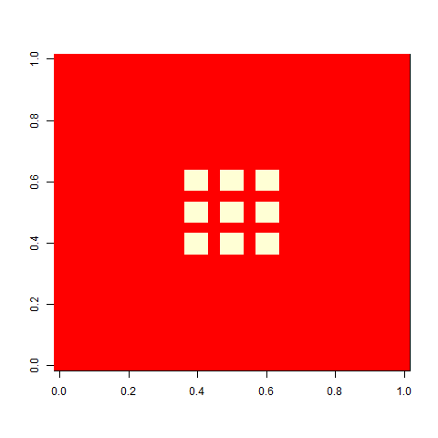
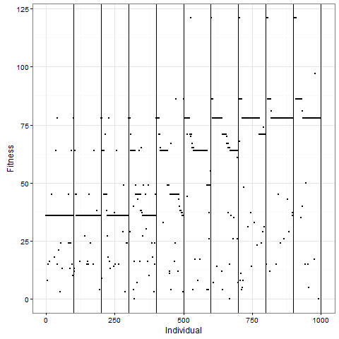
Let me now tell you that I was almost completely wrong about what happens with this pattern once you apply selection. I thought that the initial pattern of nine stable blocks (36 cells) was pretty good, and that it would be preserved for long, and that virus-like patterns (like the first animation above) would mostly have degenerated around 80. As this plot of the evolution of the number of cells in one replicate shows, I grossly underestimated this pattern. The y-axis is number of cells at time 80, and the x-axis individuals, the vertical lines separating generations. Already by generation five, most individuals do better than 36 cells in this case:

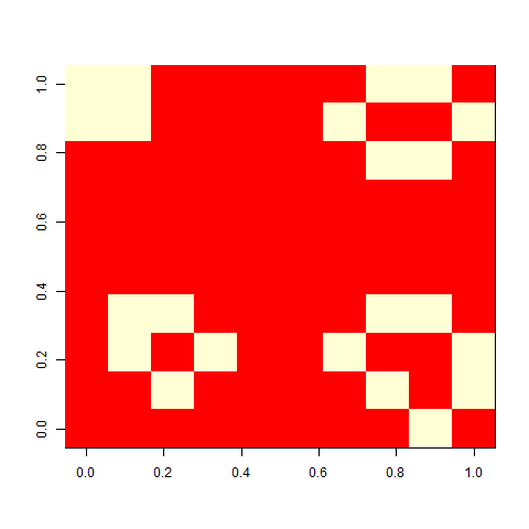
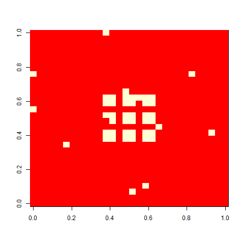
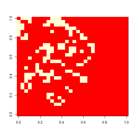
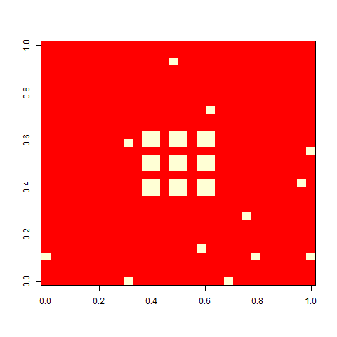
As one example, here is the starting position and the state at time 80 for a couple of individuals from generation 10 of one of my replicates:


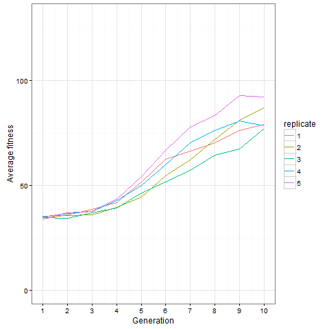
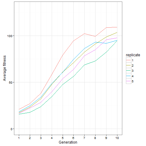
Here is how the average cell number at time 80 evolves in five replicates. Clearly, things are still going on at generation 10, not only in the replicate shown above.

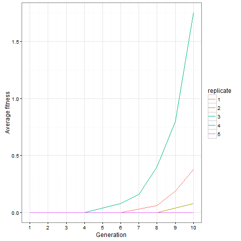
Here is the same plot for the virus pattern I showed above, i.e. the blocks but with one single added cell, fixed in the starting population. Prior genetic architecture matters. Even if the virus pattern has fewer cells than the blocks pattern at time 80, it is apparently a better starting point to quickly evolve more cells:

And finally, out of curiosity, what happens if we start with an empty 30 x 30 board?
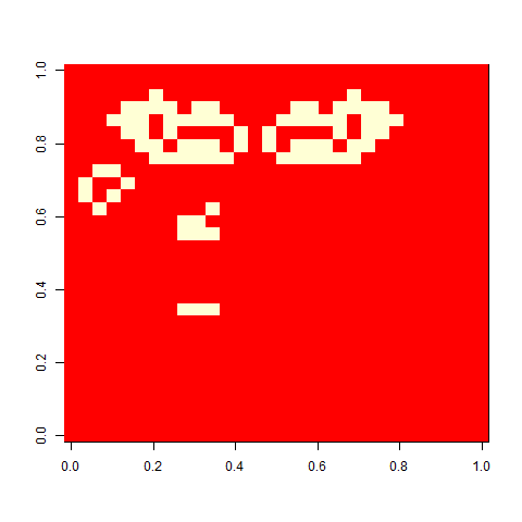
Not much. The simple still life block evolves a lot. But in my replicate three, this creature emerged. ”Life, uh, finds a way.”

Unfortunately, many of the selected patterns extended to the edges of the board, making them play not precisely the game of life, but the game of life with edge effects. I’d like to use a much bigger board and see how far patterns extend. It would also be fun to follow them longer. To do that, I would need to implement a more efficient way to update the board (this is very possible, but I was lazy). It would also be fun to select for something more complex, with multiple fitness components, potentially in conflict, e.g. favouring patterns that grow large at a later time while being as small as possible at an earlier time.
Code is on github, including functions to display and animate boards with the animation package and ImageMagick, and code for the plots. Again, the blocks_selection.R script is slow, so leave it running and go do something else.
 ,
,  and
and  before selection.
 for Aa and
  for aa. We can think of this as the probability of contributing to the next generation.
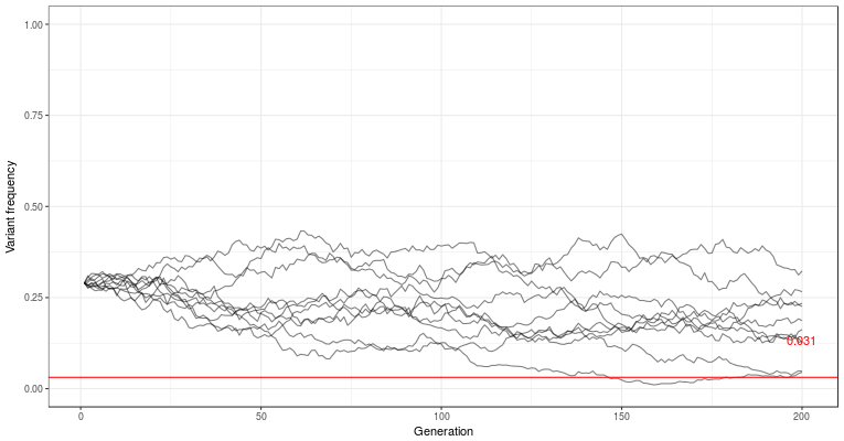
 is the mutation rate. It’s not easy to see what is going on here, but we can draw it in the graph, and see that it’s usually very small. In these small populations, where drift is a major player, the variants are often completely lost, or drift to higher frequency by chance.