Convincing myself about the Monty Hall problem

Like many others, I’ve never felt that the solution to the Monty Hall problem was intuitive, despite the fact that explanations of the correct solution are everywhere. I am not alone. Famously, columnist Marilyn vos Savant got droves of mail from people trying to school her after she had published the correct solution.

The problem goes like this: You are a contestant on a game show (based on a real game show hosted by Monty Hall, hence the name). The host presents you with three doors, one of which contains a prize — say, a goat — and the others are empty. After you’ve made your choice, the host opens one of the doors, showing that it is empty. You are now asked whether you would like to stick to your initial choice, or switch to the other door. The right thing to do is to switch, which gives you 2/3 probability of winning the goat. This can be demonstrated in a few different ways.

A goat is a great prize. Image: Casey Goat by Pete Markham (CC BY-SA 2.0)

So I sat down to do 20 physical Monty Hall simulations on paper. I shuffled three cards with the options, picked one, and then, playing the role of the host, took away one losing option, and noted down if switching or holding on to the first choice would have been the right thing to do. The results came out 13 out of 20 (65%) wins for the switching strategy, and 7 out of 20 (35%) for the holding strategy. Of course, the Monty Hall Truthers out there must question whether this demonstration in fact happened — it’s too perfect, isn’t it?

The outcome of the simulation is less important than the feeling that came over me as I was running it, though. As I was taking on the role of the host and preparing to take away one of the losing options, it started feeling self-evident that the important thing is whether the first choice is right. If the first choice is right, holding is the right strategy. If the first choice is wrong, switching is the right option. And the first choice, clearly, is only right 1/3 of the time.

In this case, it was helpful to take the game show host’s perspective. Selvin (1975) discussed the solution to the problem in The American Statistician, and included a quote from Monty Hall himself:

Monty Hall wrote and expressed that he was not ”a student of statistics problems” but ”the big hole in your argument is that once the first box is seen to be empty, the contestant cannot exchange his box.” He continues to say, ”Oh, and incidentally, after one [box] is seen to be empty, his chances are no longer 50/50 but remain what they were in the first place, one out of three. It just seems to the contestant that one box having been eliminated, he stands a better chance. Not so.” I could not have said it better myself.

A generalised problem

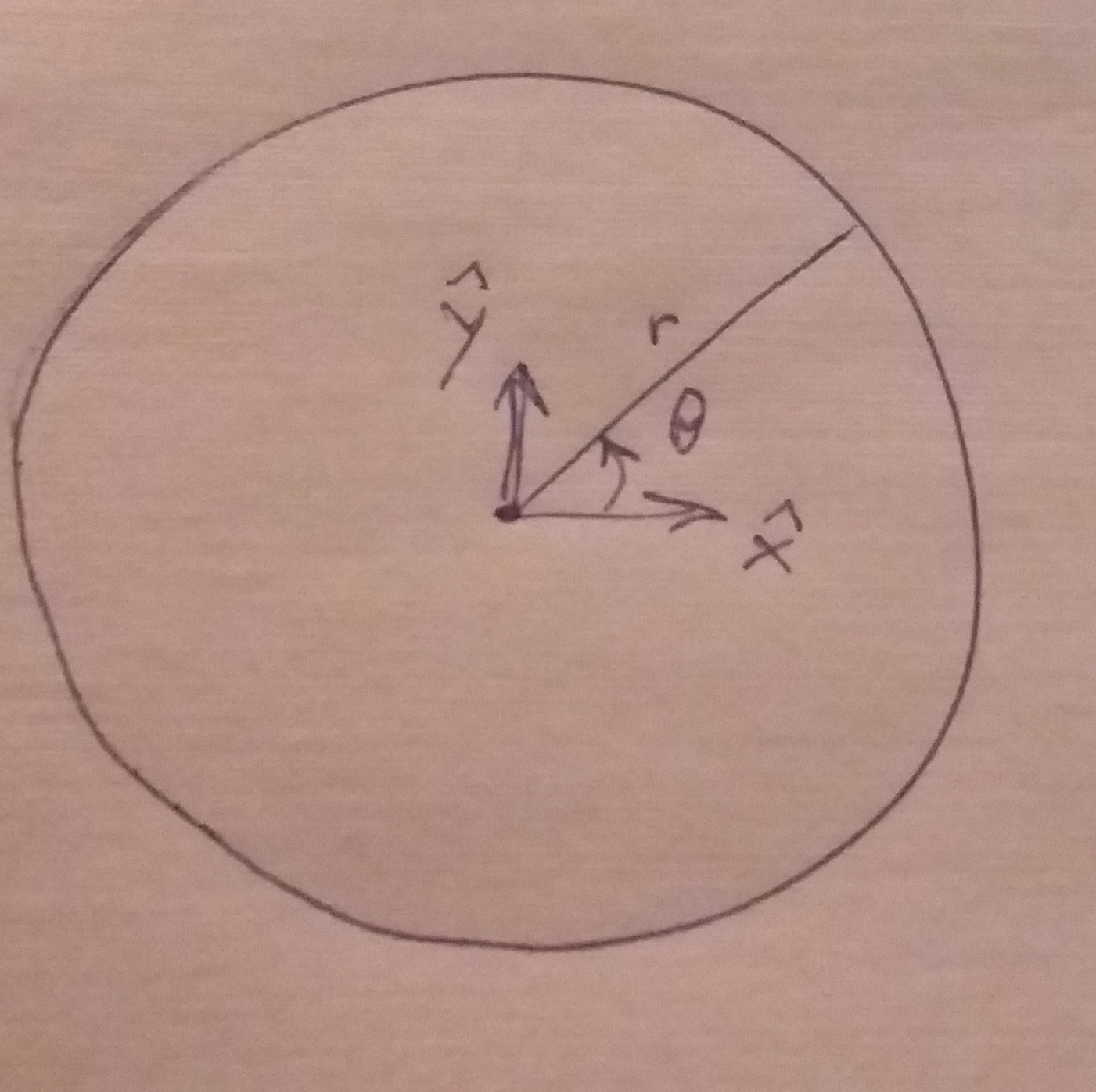
Now, imagine the same problem with a number d number of doors, w number of prizes and o number of losing doors that are opened after the first choice is made. We assume that the losing doors are opened at random, and that switching entails picking one of the remaining doors at random. What is the probability of winning with the switching strategy?

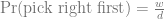
The probability of picking the a door with or without a prize is:

\Pr(\text{pick right first}) = \frac{w}{d}

\Pr(\text{pick wrong first}) = 1 - \frac{w}{d}

If we picked a right door first, we have w – 1 winning options left out of d – o – 1 doors after the host opens o doors:

\Pr(\text{win\textbar right first}) = \frac{w - 1}{d - o - 1}

If we picked the wrong door first, we have all the winning options left:

\Pr(\text{win\textbar wrong first}) = \frac{w}{d - o - 1}

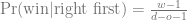
Putting it all together:

\Pr(\text{win\textbar switch}) = \Pr(\text{pick right first}) \cdot \Pr(\text{win\textbar right first}) + \\   + \Pr(\text{pick wrong first}) \cdot \Pr(\text{win\textbar wrong first}) = \\  = \frac{w}{d} \frac{w - 1}{d - o - 1} + (1 - \frac{w}{d}) \frac{w}{d - o - 1}

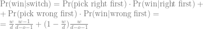
As before, for the hold strategy, the probability of winning is the probability of getting it right the first time:

\Pr(\text{win\textbar hold}) = \frac{w}{d}

With the original Monty Hall problem, w = 1, d = 3 and o = 1, and therefore

\Pr(\text{win\textbar switch}) = \frac{1}{3} \cdot 0 + \frac{2}{3} \cdot 1

Selvin (1975) also present a generalisation due to Ferguson, where there are n options and p doors that are opened after the choice. That is, w = 1, d = 3 and o = 1. Therefore,

\Pr(\text{win\textbar switch}) = \frac{1}{n} \cdot 0 + (1 - \frac{1}{n}) \frac{1}{n - p - 1} =  \frac{n - 1}{n(n - p - 1)}

which is Ferguson’s formula.

Finally, in Marilyn vos Savant’s column, she used this thought experiment to illustrate why switching is the right thing to do:

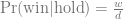
Here’s a good way to visualize what happened. Suppose there are a million doors, and you pick door #1. Then the host, who knows what’s behind the doors and will always avoid the one with the prize, opens them all except door #777,777. You’d switch to that door pretty fast, wouldn’t you?

That is, w = 1 still, d = 106 and o = 106 – 2.

\Pr(\text{win\textbar switch}) = 1 - \frac{1}{10^6}

It turns out that the solution to the generalised problem is that it is always better to switch, as long as there is a prize, and as long as the host opens any doors. One can also generalise it to choosing sets of more than one door. This makes some intuitive sense: as long as the host takes opens some doors, taking away losing options, switching should enrich for prizes.

Some code

To be frank, I’m not sure I have convinced myself of the solution to the generalised problem yet. However, using the code below, I did try the calculation for all combinations of total number of doors, prizes and doors opened up to 100, and in all cases, switching wins. That inspires some confidence, should I end up on a small ruminant game show.

The code below first defines a wrapper around R’s sampling function, which has a very annoying alternative behaviour when fed a vector of length one, to be able to build a computational version of my physical simulation. Finally, we have a function for the above formulae. (See whole thing on GitHub if you are interested.)

## Wrap sample into a function that avoids the "convenience"
## behaviour that happens when the length of x is one

sample_safer <- function(to_sample, n) {
  assert_that(n <= length(to_sample))
  if (length(to_sample) == 1)
    return(to_sample)
  else {
    return(sample(to_sample, n))
  }
}


## Simulate a generalised Monty Hall situation with
## w prizes, d doors and o doors that are opened.

sim_choice <- function(w, d, o) {
  ## There has to be less prizes than unopened doors
  assert_that(w < d - o) 
  wins <- rep(1, w)
  losses <- rep(0, d - w)
  doors <- c(wins, losses)
  
  ## Pick a door
  choice <- sample_safer(1:d, 1)
  
  ## Doors that can be opened
  to_open_from <- which(doors == 0)
  
  ## Chosen door can't be opened
  to_open_from <- to_open_from[to_open_from != choice]
  
  ## Doors to open
  to_open <- sample_safer(to_open_from, o)
  
  ## Switch to one of the remaining doors
  possible_switches <- setdiff(1:d, c(to_open, choice))
  choice_after_switch <- sample_safer(possible_switches , 1)
  
  result_hold <- doors[choice]
  result_switch <- doors[choice_after_switch]
  c(result_hold,
    result_switch)
}


## Formulas for probabilities

mh_formula <- function(w, d, o) {
  ## There has to be less prizes than unopened doors
  assert_that(w < d - o) 
  
  p_win_switch <- w/d * (w - 1)/(d - o - 1) +
                     (1 - w/d) * w / (d - o - 1) 
  p_win_hold <- w/d
  c(p_win_hold,
    p_win_switch)
}


## Standard Monty Hall

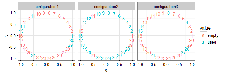
mh <- replicate(1000, sim_choice(1, 3, 1))
> mh_formula(1, 3, 1)
[1] 0.3333333 0.6666667
> rowSums(mh)/ncol(mh)
[1] 0.347 0.653

The Monty Hall problem problem

Guest & Martin (2020) use this simple problem as their illustration for computational model building: two 12 inch pizzas for the same price as one 18 inch pizza is not a good deal, because the 18 inch pizza contains more food. Apparently this is counter-intuitive to many people who have intuitions about inches and pizzas.

They call the risk of having inconsistencies in our scientific understanding because we cannot intuitively grasp the implications of our models ”The pizza problem”, arguing that it can be ameliorated by computational modelling, which forces you to spell out implicit assumptions and also makes you actually run the numbers. Having a formal model of areas of circles doesn’t help much, unless you plug in the numbers.

The Monty Hall problem problem is the pizza problem with a vengeance; not only is it hard to intuitively grasp what is going on in the problem, but even when presented with compelling evidence, the mental resistance might still remain and lead people to write angry letters and tweets.

Literature

Guest, O, & Martin, AE (2020). How computational modeling can force theory building in psychological science. Preprint.

Selvin, S (1975) On the Monty Hall problem. The American Statistician 29:3 p.134.

Peer review glossary

‘Misleading’ — not exactly as I would have written it

‘Somewhat confusing’ — using terminology from adjacent sub-subfield

‘Confusing’ — completely illegible

‘Poorly structured’ — not exactly as I would have written it

‘Conversational’ — in need of adjectives

‘Descriptive’ — using technology that isn’t fashionable anymore

‘Potentially’ — definitely

‘by a native English speaker’ — by the Microsoft Word spell checker

‘due to insufficient enthusiasm’ — because it’s trite

‘gratefully’ — begrudgingly

‘adequate’ — perfunctory

‘constructive’ — fairly polite

Clearly, obviously

This is my kind of letter to Nature:

This is a friendly suggestion to colleagues across all scientific disciplines to think twice about ever again using the words ‘obviously’ and ‘clearly’ in scientific and technical writing. These words are largely unhelpful, particularly to students, who may be counterproductively discouraged if what is described is not in fact obvious or clear to them.

Clearly, this is easier said than done. It is common writers’ advice to remove adverbs, and to a lesser extent adjectives. These words may be pointless filler words, and when they’re not, there is a risk of telling the reader what to think in a manner that seems impolite. But they also do some work to make the text flow, and prose without them can seem sterile and disconnected.

If we could also get rid of ”surprisingly”, I would be happy.

Balancing a centrifuge

I saw this cute little paper on arxiv about balancing a centrifuge: Peil & Hauryliuk (2010) A new spin on spinning your samples: balancing rotors in a non-trivial manner. Let us have a look at the maths of balancing a centrifuge.

The way I think most people (including myself) balance their samples is to put them opposite of each other, just like Peil & Hauryliuk write. However, there are many more balanced configurations, some of which look really weird. The authors generate three balanced configurations with increasing oddity, show them to researchers and ask them whether they are balanced. About half, 30% and 15% of them identified each configuration as balanced. Here are the configurations:

configuration_plot
(Drawn after their paper.)

Take a rotor in a usual bench top centrifuge. It’s a large, in itself balanced, piece of metal with holes to put microcentrifuge tubes in. We assume that all tubes have the same mass m and that the holes are equally spaced. The rotor will spin around its own axis, helping us separate samples and pellet precipitates etc. When the centrifuge is balanced, the centre of mass of the samples will be aligned with the axis of rotation. So, if we place a two-dimensional coordinate system on the axis of rotation like so,

koordinater

the tubes are positioned on a circle around it:

x_i = r \cos {\theta_i}
y_i = r \sin {\theta_i}

The angle to each position in the rotor will be

\theta(i) = \dfrac{2\pi(i - 1)}{N}

where i is the position in question, starting at 1, and N the number of positions in the rotor. Let’s label each configuration by the numbers of the positions that are occupied. So we could talk about (1, 16)30 as the common balanced pair of tubes in a 30-position rotor. (Yeah, I know, counting from 1 is a lot more confusing than counting from zero. Let’s view it as a kind of practice for dealing with genomic coordinates.)

We express the position of each tube (treated as a point mass) as a vector. Since we put the origin on the axis of rotation, these vectors have to sum to zero for the centrifuge to be balanced.

\sum \limits_{i} {m\mathbf{r_i}} = \mathbf{0}

Since the masses are equal, they can be removed, as can the radius, which is constant, and we can consider the x and y coordinates separately.

\left(\begin{array}{c} \sum \limits_{i} {\cos {\theta(i)}} \\ \sum \limits_{i} {\sin {\theta(i)}} \end{array}\right) = \left(\begin{array}{c} 0 \\ 0 \end{array}\right)

For the (1, 16)30 configuration, the vectors are

\left(\begin{array}{c} \cos {\theta(1)} \\ \sin {\theta(1)} \end{array}\right) + \left(\begin{array}{c} \cos {\theta(16)} \\ \sin {\theta(16)} \end{array}\right) = \left(\begin{array}{c} \cos {0} \\ \sin {0} \end{array}\right) + \left(\begin{array}{c} \cos {\pi} \\ \sin {\pi} \end{array}\right) = \left(\begin{array}{c} 1 \\ 0 \end{array}\right) + \left(\begin{array}{c} -1 \\ 0 \end{array}\right)

So we haven’t been deluding ourselves. This configuration is balanced. That is about as much maths as I’m prepared to do in LaTex in a WordPress blog editor. So let’s implement this in R code:

library(magrittr)
theta <- function(n, N) (n - 1) * 2 * pi / N
tube <- function(theta) c(cos(theta), sin(theta))

Now, we can look at Peil & Hauryliuk’s configurations, for instance the first (1, 11, 14, 15, 21, 29, 30)30

positions <- c(1, 11, 14, 15, 21, 29, 30)
tubes <- positions %>% lapply(theta, N = 30) %>% lapply(tube)
c(sum(unlist(lapply(tubes, function(x) x[1]))),
  sum(unlist(lapply(tubes, function(x) x[2]))))

The above code 1) defines the configuration; 2) turns positions into angles and then tube coordinates; and 3) sums the x and y coordinates separately. The result isn’t exactly zero (for computational reasons), but close enough. Putting in their third configuration, (4, 8, 14, 15, 21, 27, 28)30, we again get almost zero. Even this strange-looking configuration seems to be balanced.

I’m biased because I read the text first, but if someone asked me, I would have to think about the first two configurations, and there is no way I would allow a student to run with the third if I saw it in the lab. That conservative attitude, though not completely scientific, might not be the worst thing. Centrifuge accidents are serious business, and as the authors note:

Finally, non-symmetric arrangement (Fig. 1C) was recognized as balanced by 17% of researchers. Some of these were actually calculating moment of inertia, i.e. were coming to solution knowingly, the rest where basically guessing. The latter should be banished from laboratory practice, since these people are ready to make dangerous decisions without actual understanding of the case, which renders them extremely dangerous in the laboratory settings.

(Plotting code for the first figure is on Github.)

Hönan och ägget

På samma tema som igår, nämligen ofta ställda men lite aviga frågor: vad kom först, hönan eller ägget? Ägget, naturligtvis. Så många av hönans både nära och avlägsna släktingar lägger ägg, vilket betyder att deras gemensamma släktingar med största säkerhet lade ägg och alltså måste ägget vara oerhört, oerhört mycket äldre än hönan som art. Vad kom först, hönan eller hönsägget? Hönsägget, kanske. Det är inte helt enkelt att definiera arter, men om vi föreställer oss att det finns någon punkt där en individer i en population av för-höns ackumulerat tillräckligt många hönslika egenskaper för att vara det vi skulle kalla en höns så började de i alla fall sina liv som ägg. Alltså fanns hönsägg innan det fanns vuxna höns. Eller så är hönor bara en sorts teoretiska efterhandskonstruktioner människor använder för att göra naturens röra hanterbar.

Så kristdemokrater har mest sex, säger ni?

Nja. Två som röstar på kristdemokraterna har mycket sex.

Rplot02

Aftonbladet har köpt någon sorts undersökning om svenskarnas sexvanor. Hoppas det var en god investering; jag tror i alla fall den har genererat löpsedlar ett par dagar. Nu har turen kommit till politiska sympatier och sex. Data finns på United minds hemsida. Kristdemokraterna har alltså minst stickprovsstorlek, men hela två som uppgivit att de haft sex fler än femtio gånger de sista 30 dagarna. Sådana extrema värden kan dra iväg medelvärdet ganska ordentligt, som till exempel i Aftonbladets diagram, vilket därför är rätt missvisande.

Weird juxtapositions happen when you import Wikipedia

The network is available on IntegromeDB public database (http://integromedb.org) under the present manuscript title.

So I went there:

integromedb

Apparently, typing in journal article titles was not what the search field was for. Couldn’t find the network either, but the article is still in provisional pdf form so that may be the reason.

Dragana Stanley, Nathan S Watson-Haigh, Christopher JE Cowled, Robert J Moore. (2013) Genetic architecture of gene expression in the chicken. BMC Genomics 14

Om någon av mina studenter läser det här

Så har ni förhoppningsvis gjort er förtjänta av en välbehövlig paus. Jag vill inte uppmuntra till dryckenskap eller kille-med-gitarrbeteende, men den här söta nördiga videon innehåller i alla fall några kul upplysningar om osmoreglering, cellsignalering samt vår favoritorganism från labb B1.

(Mina och mina … Studenterna är väl sina egna. Dessutom är jag bara med på labbar och hoppar in på ett par föreläsningar. Men det tycker jag är fullt tillräckligt mandat att föreslå youtubeklipp i alla fall.)