@sweden recap

So, a couple of weeks ago I tweeted from the @sweden account. This is a short recap of some things that were said, and a few links that I promised people. Overall I think it went pretty well. I didn’t tweet as much as some other curators, but much much more than I usually do. This also meant I did spend my lunch and coffee breaks looking at my phone. My tweets are collected here, if for some reason you’d care to read them.

Of course, tweeting from a rotating curation account is very different from the way I normally use Twitter. First, I read much more than I write. One of the main purposes of Twitter, for me, is to get a steady stream of links to read. That doesn’t really work on an account that follows much more and entirely different people. A lot of what I wrote was prepared monologue, but I don’t think that’s necessarily a bad thing. I follow a lot of people on Twitter for their monologues. Also, thankfully, a lot of people asked me questions! Another thing that struck me is that so few people were unpleasant. There were a few extreme right folks who wanted me to retweet their racist tweets, but only a few. Then, a few felt the need to tell me that I’m utterly boring, which is fine. Someone lamented the fact that all curators are uneducated about the proper use of Twitter (it’s probably to build your personal brand or something). Also, a certain Swedish celebrity got put on ignore so I wouldn’t have to see him tagging each tweet with ”@sweden”. But that was pretty much all.

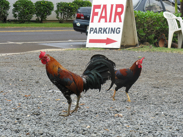
I talked quite a bit about my research. I spent more or less a full day on the chicken comb as a sexual ornament and genetics of comb mass. We discussed domestication as an evolutionary process, tonic immobility, and how to measure gene expression for eQTL mapping. I also wrote about Kauai feral chickens … And what I actually do in a day nowadays, that is: writing R code.

I got a question about what to say to your creationist friend. I think this depends on what the creationist friend believes and what their objections to evolution are. Unfortunately, I don’t think there is a simple knock-down argument against all forms of creationism, except that evolution works really well and has a lot of evidence going for it. I certainly don’t think it will do to rely on methodological naturalism and say that ”creation would be a supernatural event and outside the scope of science”. First, because I don’t think that is how science works. Say if unicorns, miraculous healing, and species popping into existence without relation to other species were actually part of the world, wouldn’t we want to study that? Second, that will never convince anyone, except of the irrelevance of science to their worldview.

But I think there are a handful of things that creationists often take issue with. First, some don’t believe in sequence variants creating new functions. This is often described with slogans about information, and how it cannot be created by random mutation. I don’t think ”sequence information” is a particularly useful concept, and would much prefer to talk about function and adaptation. That is what is important, after all, organisms acquiring new adaptations. It turns out, new functions arising can be observed, particularly in microorganisms. Some really fun and well-studied example occur in the Long Term Evolution Experiment; see Richard Lenski’s blog which has explanatory posts and links to papers.

Second, the formation of species come up a lot in these discussions. This is a bit tricky, because it’s not always clear what constitutes different species. The definition most people have heard is probably that individuals belong to different species if they cannot have fertile offspring. But just think of asexually reproducing organisms. There, individuals belong to different species if they’re sufficiently different. So we already have what is needed to understand the formation of species in the evolution of new functions. When it comes to sexually reproducing organisms, there are examples of the evolution of reproductive isolation — cases where it seems to be ongoing or to have happened recently. (See for instance this paper on hybrid incompatibility in Mimulus guttatus; I have blogged about it, but only in Swedish)

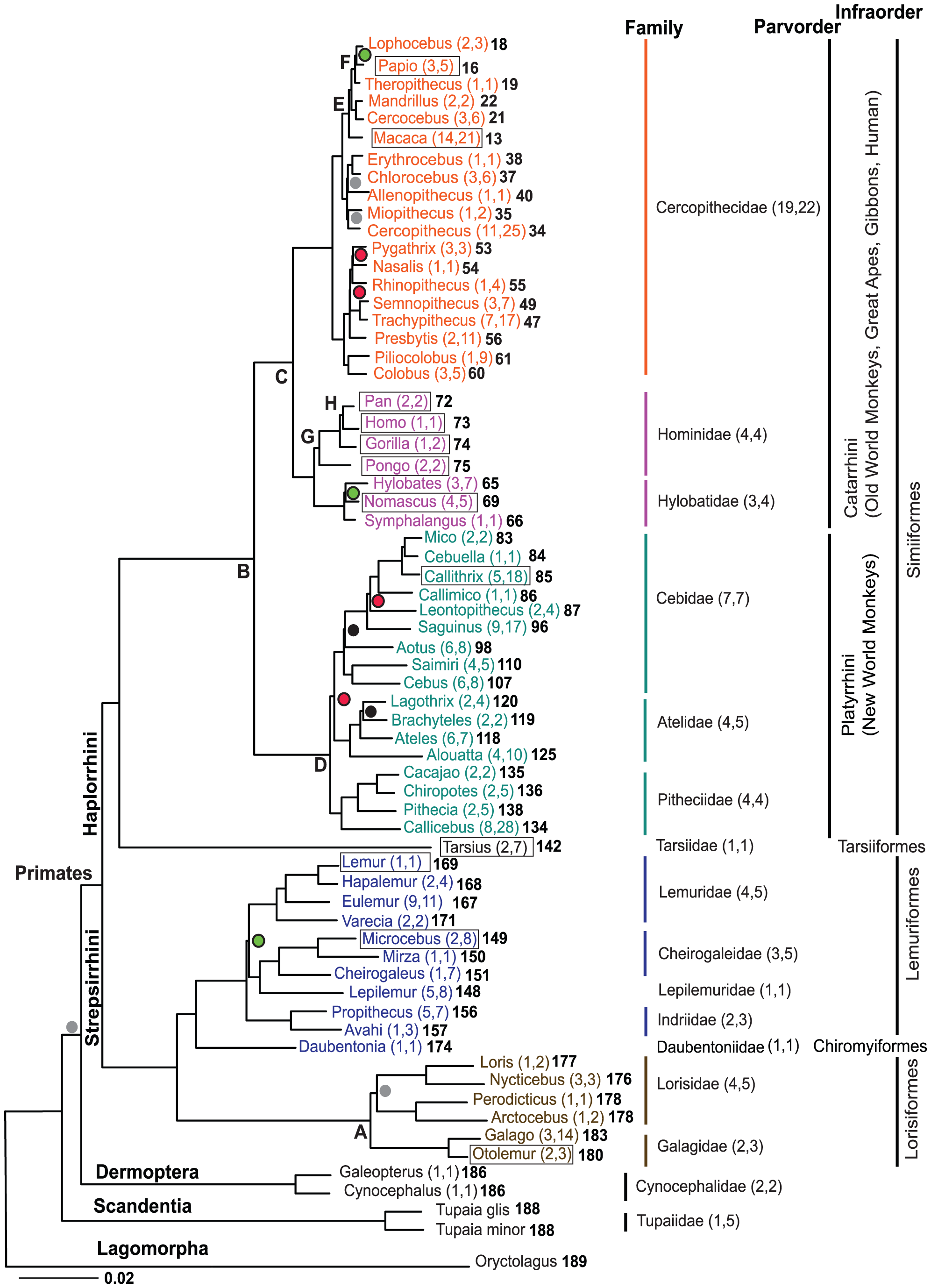
Third, there is the question of relatedness between species. In particular, some creationists really hate the idea that humans are apes. I think it is important to emphasize a couple of things that evolution does not say about humans and other apes. By the way, this isn’t just confusing for creationists, but for everyone. Evolution does not mean that humans descend from extant apes. Look at this phylogenetic tree from Perelman & al 2011. This is just like a family tree, but of populations: we see how chimps and humans have a recent common ancestor population. This is different than claiming that we would descend from extant chimps. Of course, chimps have also changed since the common ancestor, although not in the same ways as humans. (Again, I’ve written about this before in Swedish.)

journal.pgen.1001342.g001

Speaking of unicorns, I of course celebrated unicorn Friday:

Someone asked whether you can keep fruit flies for amateur genetics at home. That should be quite possible, and I don’t see any real problems with it either. The fruit fly community has really strong culture of classical genetics with crosses and stocks. I don’t know if stock centres would deliver to private customers, but I don’t see why they wouldn’t — except for transgenic flies. It turned out, however, that transgenic flies was actually what the person asking was after. And of course, I can’t recommend that. I must say, I have mixed feelings about do-it-yourself biotechnology. On the one hand, some home molecular biology should be possible and rewarding. On the other hand, a lot of things routinely used in molecular labs are actually really dangerous if misused, and not just for the user. For example, when making any type of construct in transgenic bacteria, antibiotics and antibiotic resistance genes are the standard screening markers. They are used to pick out the bacteria that have incorporated the piece of DNA you care about. This is not the kind of stuff you want to use without proper containment. So, in the fly example, you would not only have to handle the flies, but also transgenic antibiotic resistant bacteria safely and legally. Then again, a lot of the genetics I care about does not involve any of that, and could very well be done in a basement.

The @sweden account caught me under a teaching week; otherwise, all of my photos would’ve been my computer, my pen and my coffee mug. Now I got to walk the followers through agarose gel electrophoresis and a little transformation of bacteria:

And, finally, Swedish spring:

Paper: ”Mixed ancestry and admixture in Kauai’s feral chickens: invasion of domestic genes into ancient Red Junglefowl reservoirs”

We have a new paper almost out (now in early view) in Molecular Ecology about the chickens on the Pacific island Kauai. These chickens are pretty famous for being everywhere on the island. Where do they come from? If you use your favourite search engine you’ll find an explanation with two possible origins: ancient wild birds brought over by the Polynesians and escaped domestic chickens. This post on Kauaiblog is great:

Hawaii’s official State bird is the Hawaiian Goose, or Nene, but on Kauai, everyone jokes that the “official” birds of the Garden Island are feral chickens, especially the wild roosters.

Wikepedia says the “mua” or red jungle fowl were brought to Kauai by the Polynesians as a source of food, thriving on an island where they have no real predators. /…/
Most locals agree that wild chickens proliferated after Hurricane Iniki ripped across Kauai in 1992, destroying chicken coops and releasing domesticated hens, and well as roosters being bred for cockfighting. Now these brilliantly feathered fowl inhabit every part of this tropical paradise, crowing at all hours of the day and night to the delight or dismay of tourists and locals alike.

In this paper, we look at phenotypes and genetics and find that this dual origin explanation is probably true.

jeff_trimble_kauai_chickens_cc_by_nc_sa

(Chickens on Kauai. This is not from our paper, but by Jeff Trimble (cc:by-sa-nc) published on Flickr. There are so many pretty chicken pictures there!)

Dom, Eben, and Pamela went to Kauai to photograph, record to and collect DNA from the chickens. (I stayed at home and did sequence bioinformatics.) The Kauai chickens look and sound like mixture of wild and domestic chickens. Some of them have the typical Junglefowl plumage, and other have flecks of white. Their crows vary in the length of the characteristic fourth syllable. Also, some of them have yellow legs, a trait that domestic chickens seem to have gotten not from the Red but from the Grey Junglefowl.

We looked at DNA sequences by massively parallel (SOLiD) sequencing of 23 individuals. We find mitochondrial sequences that fall in two haplogroups: E and D. The presence of the D haplogroup, which is the dominating one in ancient DNA sequences from the Pacific, means that there is a Pacific component to their ancestry. The E group, on the other hand, occurs in domestic chickens. It also shows up in some ancient DNA samples from the Pacific, but not from Kauai (and there is a scientific debate about these sequences). The nuclear genome analysis is pretty inconclusive. I think what we would need is some samples of possible domestic source populations (Where did the escapee  chickens came from? Are there other traditional domestic sources?) and a better sampling of Red Junglefowl to make better sense of it.

When we take the plumage, vocalisation and mitochondrial DNA together, it looks like this is a feral admixed population of either Red Junglefowl or traditional Pacific chickens mixed with domestics. A very interesting population indeed.

Kenneth Chang wrote about the paper in New York Times; includes quotes from Eben and Dom.

E Gering, M Johnsson, P Willis, T Getty, D Wright (2015) Mixed ancestry and admixture in Kauai’s feral chickens: invasion of domestic genes into ancient Red Junglefowl reservoirs. Molecular ecology

Morning coffee: cost per genome

I recently heard this thing referred to as ”the most overused slide in genomics” (David Klevebring). It might be: what it shows is some estimate of the cost of sequencing a human genome over time, and how it plummets around 2008. Before that, the curve is Sanger sequencing, and then the costs show second generation sequencing (454, Illumina and SOLiD).

cost_genome

The source is the US National Human Genome Research Institute, and they’ve put some thought into how to estimate costs so that machines, reagents, analysis and people to do the work are included and that the different platforms are somewhat comparable. One must first point out that downstream analysis to make any sense of the data (assembly and variant calling) isn’t included. But the most important thing that this graph hides, even if the estimates of the cost would be perfect, is that to ”sequence a genome” means something completely different in 2001 and 2015. (Well, with third generation sequencers that give long reads coming up, the old meaning might come back.)

For data since January 2008 (representing data generated using ‘second-generation’ sequencing platforms), the ”Cost per Genome” graph reflects projects involving the ‘re-sequencing’ of the human genome, where an available reference human genome sequence is available to serve as a backbone for downstream data analyses.

The human genome project was of course about sequencing and assembling the genome into high quality sequences. Very few of the millions of human genomes resequenced since are anywhere close. As people in the sequencing loop know, resequencing with short reads doesn’t give you a genome sequence (and neither does trying to assemble a messy eukaryote genome with short reads only). It gives you a list of variants compared to the reference sequence. The usual short read business has no way of detect anything but single nucleotide variants and small indels. (And the latter depends … Also, you can detect copy number variants, but large scale structural variants are mostly off the table.) Of course, you can use these edits to reconstruct a consensus sequence from the reference, but it would be a total lie.

Again, none of this is news for people who deal with sequencing, and I’m not knocking second-generation sequencing. It’s very useful and has made a lot of new things possible. It’s just something I think about every time I see that slide.

R in genomics @ SciLifeLab, Solna

Dear diary,

I went to the Stockholm R useR group meetup on R in genomics at the Stockholm node of SciLifeLab. It was nice. If I had worked a bit closer I would attend meetups all the time. I even got to be pretentious with my notebook while waiting for the train.

blog_pretentious

The speakers were:

Jakub Orzechowski Westholm on R and genomics in general. He demonstrated genome browser-style tracks with Gviz, some GenomicRanges, and a couple of common plots of gene expression data. I have been on the fence about what package I should use for drawing genes and variants along the genome. I should play with Gviz.

Daniel Klevebring on clinical sequencing and how he uses R (not that much) in sequencing pipelines aimed at targeting the right therapy to patients based on the mutations in their cancer cells. He mentioned some getopt snippets for getting R to play nicely on the command line, which is something I should definitely try more!

Finally, Arvind Singh Mer on predictive modelling for clinical genomics (like the abovementioned ClinSeq data). He showed the caret package for machine learning, with an elastic net regression.

I don’t know the rest of the audience, so maybe the choice to gear talks towards the non-bio* person was spot on, but that made things a bit less interesting for me. For instance, in Jakub’s talk about gene expression, I would’ve preferred more about the messy stuff: how to make that nice gene-by-sample matrix in the first place, and if R can be of any help in that process; also, in the other end, what models one would use after that first pass of visualisation. But this isn’t a criticism of the presenters — time and complexity constraints apply. (If I was asked to present how I use R any demos would be toy analyses of clean datasets. That is the way these things go.)

We also heard repeated praise for and recommendations of the hadleyverse and data.table. I’m not a data.tabler myself, but I probably should be. And I completely agree about the value of dplyr — there’s this one analysis where a couple of lines with dplyr changed it from ”argh, do I have to rewrite this in C?” to being workable. I think we also saw all the three plotting systems: base graphics, ggplot2 and lattice in action.

Finding the distance from ChIP signals to genes

I’ve had a couple of months off from blogging. Time for some computer-assisted biology! Robert Griffin asks on Stack Exchange about finding the distance between HP1 binding sites and genes in Drosophila melanogaster.  We can get a rough idea with some public chromatin immunoprecipitation data, R and the wonderful BEDTools.

Finding some binding sites

There are indeed some ChIP-seq datasets on HP1 available. I looked up these ones from modENCODE: modENCODE_3391 and modENCODE_3392, using two different antibodies for Hp1b in 16-24 h old embroys. I’m not sure since the modENCODE site doesn’t seem to link datasets to publications, but I think this is the paper where the results are reported: A cis-regulatory map of the Drosophila genome (Nègre & al 2011).

What they’ve done, in short, is cross-linking with formaldehyde, sonicate DNA into fragments, capture fragments with either of the two antibodies and sequence those fragments. They aligned reads with Eland (Illumina’s old proprietary aligner) and called peaks (i.e. regions where there is a lot of reads, which should reflect regions bound by Hp1b) with MACS. We can download their peaks in general feature format.

I don’t know whether there is any way to make completely computation predictions of Hp1 binding sites but I doubt it.

Some data cleaning

The files are available from ftp, and for the below analysis I’ve unzipped them and called them modENCODE_3391.gff3 and modENCODE_3392.gff3. GFF is one of all those tab separated text files that people use for genomic coordinates. If you do any bioinformatics type work you will have to convert back and forth between them and I suggest bookmarking the UCSC Genome Browser Format FAQ.

Even when we trust in their analysis, some processing of files is always required. In this case, MACS sometimes outputs peaks with negative start coordinates in the beginning of a chromosome. BEDTools will have none of that, because ”malformed GFF entry at line … Start was greater than end”. In this case, it happens only at a few lines, and I decided to set those start coordinates to 1 instead.

We need a small script to solve that. As I’ve written before, any language will do, but I like R and tend to do my utility scripting in R (and bash). If the files were incredibly huge and didn’t fit in memory, we’d have to work through the files line by line or chunk by chunk. But in this case we can just read everything at once and operate on it with vectorised R commands, and then write the table again.

modENCODE_3391 <- read.table("modENCODE_3391.gff3", stringsAsFactors=F, sep="\t")
modENCODE_3392 <- read.table("modENCODE_3392.gff3", stringsAsFactors=F, sep="\t")

fix.coord <- function(gff) {
  gff$V4[which(gff$V4 < 1)] <- 1
  gff
}

write.gff <- function(gff, file) {
  write.table(gff, file=file, row.names=F, col.names=F,
              quote=F, sep="\t")
}

write.gff(fix.coord(modENCODE_3391), file="cleaned_3391.gff3")
write.gff(fix.coord(modENCODE_3392), file="cleaned_3392.gff3")

Flybase transcripts

To find the distance to genes, we need to know where the genes are. The best source is probably the annotation made by Flybase, which I downloaded from the Ensembl ftp in General transfer format (GTF, which is close enough to GFF that we don’t have to care about the differences right now).

This file contains a lot of different features. We extract the transcripts and find where the transcript model starts, taking into account whether the transcript is in the forward or reverse direction (this information is stored in columns 4, 5 and 7 of the GTF file). We store this in a new GTF file of transcript start positions, which is the one we will feed to BEDTools:

ensembl <- read.table("Drosophila_melanogaster.BDGP5.75.gtf",
                      stringsAsFactors=F, sep="\t")

transcript <- subset(ensembl, V3=="transcript")
transcript.start <- transcript
transcript.start$V3 <- "transcript_start"
transcript.start$V4 <- transcript.start$V5 <- ifelse(transcript.start$V7 == "+",
                                                     transcript$V4, transcript$V5)

write.gff(transcript.start, file="ensembl_transcript_start.gtf")

Finding distance with BEDTools

Time to find the closest feature to each transcript start! You could do this in R with GenomicRanges, but I like BEDTools. It’s a command line tool, and if you haven’t already you will need to download and compile it, which I recall being painless.

bedtools closest is the command that finds, for each feature in one file, the closest feature in the other file. The -a and -b flags tells BEDTools which files to operate on, and the -d flag that we also want it to output the distance. BEDTools writes output to standard out, so we use ”>” to capture it in a text file.

Here is the bash script. I put the above R code in clean_files.R and added it as an Rscript line at the beginning, so I could run it all with one file.

#!/bin/bash
Rscript clean_files.R

bedtools closest -d -a ensembl_transcript_start.gtf -b cleaned_3391.gff3 \
    > closest_element_3391.txt
bedtools closest -d -a ensembl_transcript_start.gtf -b cleaned_3392.gff3 \
    > closest_element_3392.txt

Some results

With the resulting file we can go back to R and ggplot2 and draw cute graphs like this, which shows the distribution of distances from transcript to Hp1b peak for protein coding and noncoding transcripts separately. Note the different y-scales (there are way more protein coding genes in the annotation) and the 10-logarithm plus one transformation on the x-axis. The plus one is to show the zeroes; BEDTools returns a distance of 0 for transcripts that overlap a Hp1b site.

closest_3391 <- read.table("~/blogg/dmel_hp1/closest_element_3391.txt", header=F, sep="\t")

library(ggplot2)
qplot(x=log10(V19 + 1), data=subset(closest_3391, V2 %in% c("protein_coding", "ncRNA"))) +
  facet_wrap(~V2, scale="free_y")

distance_hist

Or by merging the datasets from different antibodies, we can draw this strange beauty, which pretty much tells us that the antibodies do not give the same result in terms of the closest feature. To figure out how they differ, one would have to look more closely into the genomic distribution of the peaks.

closest_3392 <- read.table("~/blogg/dmel_hp1/closest_element_3392.txt", header=F, sep="\t")

combined <- merge(closest_3391, closest_3392,
                  by.x=c("V1", "V2","V4", "V5", "V9"),
                  by.y=c("V1", "V2","V4", "V5", "V9"))

qplot(x=log10(V19.x+1), y=log10(V19.y+1), data=combined)

between_antibodies

(If you’re wondering about the points that end up below 0, those are transcripts where there are no peaks called on that chromosome in one of the datasets. BEDTools returns -1 for those that lack matching features on the same chromosome and R will helpfully transform them to -Inf.)

About the DGRP

The question mentioned the DGRP. I don’t know that anyone has looked at ChIP in the DGRP lines, but wouldn’t that be fun? Quantitative genetics of DNA binding protein variation in DGRP and integration with eQTL … What one could do already, though, is take the interesting sites of Hp1 binding and overlap them with the genetic variants of the DGRP lines. I don’t know if that would tell you much — does anyone know what kind of variant would affect Hp1 binding?

Happy hacking!

Journal club of one: ”Genome-wide association of foraging behavior in Drosophila melanogaster fails to support large-effect alleles at the foraging gene” (preprint)

This preprint was posted on bioRxiv and Haldane’s sieve. It tells the story of one of the best known genetic variants affecting behaviour, the foraging gene in Drosophila melanogaster. for is still a nice example of a large-effect variant causing (developmentally) pleiotropic effects. However, Turner & al present evidence questioning whether for has any substantial effect in natural populations of flies. I think it’s self-evident why I’m interested.

They look at previous evidence for foraging as a quantitative trait gene in files sampled from natural populations and perform genome-wide association and population genetic tests with 35 DGRP lines, finding nothing at the for locus.

Comments:

(Since this is a preprint, I will feel free to suggest what I think could be improvements to the manuscript. Obviously, these are just my opinions.)

I’m not convinced one can really separate a unimodal from a bimodal distribution with 36 data points? Below are a few histograms simulated from a mixture of two normal distributions where 25 samples are ”rovers” and 11 ”sitters”.

bimodal

For fun, I also tested for normality with the Shapiro-Wilks’ test as the authors did, and about half of 1000 tests reject. My histograms should not be overinterpreted; I just generated two normal distributions with means log10(2.66) and log10(1.3) with standard deviations 0.1. I don’t know the actual standard deviations of the forS and forR reference strains. Of course, when the standard deviation is small enough, the distributions clearly separate and Shapiro-Wilks’ test will reject.

Power is difficult, but in this case the authors are looking at a well-known effect. They should be able to postulate some reasonable effect-sizes given the literature and the difference between the reference strains and make sure that they’re actually powered to detect it. 35 individuals for a GWAS is not much. They may still have good power to detect a effect of the size expected at for, at least in the single-point test, but it would be nice to demonstrate it. Power feels particularly pertinent as the authors claim to find evidence of absence. The same thing should apply to the population genetic tests, though it’s probably harder to know what effects to expect there.

The authors discuss alternative interpretations, and mention  the fact that in their hands the reference strains did not travel nearly as long as in previous experiments. How likely is it, though, that the variant isn’t segregating in Raleigh but in the populations previously sampled?

Literature

Thomas Turner, Christopher C Giauque, Daniel R Schrider, Andrew D Kern. (2014) Genome-wide association of foraging behavior in Drosophila melanogaster fails to support large-effect alleles at the foraging gene. Preprint on bioaRxiv. doi: 10.1101/004325

Interactions between genetic and epigenetic

More speculation about epigenetics and ways that epigenetic mechanisms of gene regulation could contribute to differences between individuals. Many cases, both in plants and animals, have to do with transposable elements, which makes a lot of sense since DNA methylation is involved in silencing the expression of transposable elements. Think about genetical genomics studies such as Gibbs & al (2010), where gene expression and DNA methylation is mapped to genomic regions. First, when expression QTL and methylation QTL coincide, it might be a good idea to start looking for transposable element insertions. Finding them are not as easy as finding SNPs, but hopefully, there will be SNPs tagging the actual variant and DNA methylation will spread outside of the inserted element to CpGs that are being typed. The element itself could of course work as a promoter, but it could also spread methylation into regulatory sequences of the gene, suppressing expression, or increase expression by changing the effect of an insulator.

Second, apparently the DNA methylation of transposable elements can sometimes be variable. This is the case with axin fused, Cabp-IAP and the agouti epialleles (Druker & al 2004; Vasicek & al 1997; Morgan & al 1999); among mice that carry the insertion there is DNA methylation variation causing phenotypic differences. This means that in populations where the insertion segregates, there should be a DNA methylation by gene interaction in the effect on the phenotype. I think that is fun, and I’d like to see someone find that in a mapping study. It might make things more difficult, though. The methylation–gene expression association might be hard to detect because it only exists in one of the alleles.

Third, maybe that is actually how a DNA methylation variant might escape reprogramming. Since some transposable elements are among the sequences that are not demethylated after fertilisation, and if that effect also applies to the newly inserted copy of the transposable element, our hypothetical regulatory methylation difference might be preserved through meiosis that way.

Literature

Gibbs, J. R., van der Brug, M. P., Hernandez, D. G., Traynor, B. J., Nalls, M. A., Lai, S. L., … & Singleton, A. B. (2010). Abundant quantitative trait loci exist for DNA methylation and gene expression in human brain. PLoS genetics, 6(5), e1000952.

Morgan, H. D., Sutherland, H. G., Martin, D. I., & Whitelaw, E. (1999). Epigenetic inheritance at the agouti locus in the mouse. Nature genetics, 23(3), 314-318.

Vasicek, T. J., Zeng, L. I., Guan, X. J., Zhang, T., Costantini, F., & Tilghman, S. M. (1997). Two dominant mutations in the mouse fused gene are the result of transposon insertions. Genetics, 147(2), 777-786.

Druker, R., Bruxner, T. J., Lehrbach, N. J., & Whitelaw, E. (2004). Complex patterns of transcription at the insertion site of a retrotransposon in the mouse. Nucleic acids research, 32(19), 5800-5808.

”Made obvious by our use of contraceptives”

I recently reread part of The Selfish Gene. The introduction to the 30th anniversary edition is great fun. For one thing, Dawkins expresses doubts about the word ”selfish” in the title, and ponders whether he should have called it the Immortal or Cooperative gene instead. That feels very ironic, and I for one think that he made the right choice. It also contains this nugget:

Our brains have evolved to a point where we are capable of rebelling against our selfish genes. The fact that we can do so is made obvious by our use of contraceptives. The same principle can and should work on a larger scale.

Bibliometrics and I

Dear diary,

I’m attending a course about scientific publishing, and the other day there was lecture about bibliometrics by Lovisa Österlund and David Lawrence from the Linköping University library. I don’t think I know anyone who particularly likes bibliometrics, but I guess it makes sense that if one needs to evaluate research without trying to understand what it is about there are only citations, the reputation of the publication channel and the cv of the researcher to look at. I imagine it’s a bit like reviewing a novel in a language one doesn’t know. A couple of things occured to me, though.

What to do when different instruments of evaluation give different results? Take the two papers (so far) published during my PhD: they both deal with the genetics of chicken comb size; one is published in PLOS Genetics and one in Molecular Ecology. If we look at journal impact factors (and we shouldn’t, but say that we do), PLOS Genetics comes out ahead with an impact factor of 8.5 against 6.3. For those that do not know this about it, journal impact factor is the mean number of citations for papers in that journal the last two years calculated by Thomson Reuters in their own secret way. However, Linköping University has for some reason decided to use the Norwegian index for evaluating publication channels. I don’t know why, and I don’t think it matters that much for me personally, since the system will change soon and I will finish in about a year and a half. In the Norwegian system journals are ranked as level one or two, where two is better and is supposed to represent the top 20% of that subject area. According to their database, Molecular ecology is level 2, while PLOS Genetics is level 1. The source of the discrepancy is probably that PLOS Genetics is counted as biomedicine, while Molecular Ecology is biology, according to the Norwegian database.

They also mentioned Altmetrics, and I don’t know what to make of it. On one hand, I guess it’s good to keep tabs on social media. On the other hand, what do numbers of tweets really tell you, except that one of the authors has a Twitter account? One of the examples in the lecture was the metrics page for this paper that I happen to be a contributor to. It is actually pretty strange. It shows three tweets or 11 tweets, depending on where on the page you look. Also, when I accessed this page earlier today it linked a blog. Now it doesn’t. That says something about the ephemeral nature of internet media. Regardless, when I first saw the page I thought perhaps the metrics page had picked up on my post about the paper, but that was not the case. I don’t know how altmetric.com define a ”science blog”, maybe the blog has to be listed on some aggregation site or another, and I’m not pretending my post is particularly insightful or important. Still it’s a little strange that the altmetrics page doesn’t list a post by one of the authors about the paper, but listed a post that referred to the paper with only two sentences and was mistaken about the conclusion.

Morning coffe: ”epigenetics” is also ambiguous

IMG_20140228_175448

I believe there is an analogy between the dual meaning of the word ”gene” and two senses of epigenetics, that this distinction is easy to get wrong and that it contributes to the confusion about the meaning of epigenetics. Gene can mean a sequence that has a name and a function, or it can mean a genetic variant. I sometimes, half-jokingly, call this genetics(1) and genetics(2). The order is wrong from a historical perspective, since the study of heritable variation predates the discovery of molecular genes. The first deals with the function of sequences and their products. The second deals with differences between individuals carrying different variants.

The same can be said about epigenetics. On one hand there is epigenetics(1), aiming to understand the normal function of certain molecular features, i.e. gene regulatory states that can be passed on through cell division. On the other hand, epigenetics(2) aims to explain individual variation between individuals that differ not in their DNA sequence but in other types of heritable states. And the recurring reader knows that I think that, since a lot of genetics(2) makes no assumptions about the molecular nature of the variation it studies, it will mostly work even if some of these states turn out to be epigenetic. In that sense, epigenetics(2) is a part of genetics.