Journal club: ”Template plasmid integration in germline genome-edited cattle”

(This time it’s not just a Journal Club of One, because this post is based on a presentation given at the Hickey group journal club.)

The backstory goes like this: Polled cattle lack horns, and it would be safer and more convenient if more cattle were born polled. Unfortunately, not all breeds have a lot of polled cattle, and that means that breeding hornless cattle is difficult. Gene editing could help (see Bastiaansen et al. (2018) for a model).

In 2013, Tan et al. reported taking cells from horned cattle and editing them to carry the polled allele. In 2016, Carlson et al. cloned bulls based on a couple of these cell lines. The plan was to use the bulls, now grown, to breed polled cattle in Brazil (Molteni 2019). But a few weeks ago, FDA scientists (Norris et al 2019) posted a preprint that found inadvertent plasmid insertion in the bulls, using the public sequence data from 2016. Recombinetics, the company making the edited bulls, conceded that they’d missed the insertion.

”We weren’t looking for plasmid integrations,” says Tad Sonstegard, CEO of Recombinetics’ agriculture subsidiary, Acceligen, which was running the research with a Brazilian consulting partner. ”We should have.”

Oops.

For context: To gene edit a cell, one needs to bring both the editing machinery (proteins in the case of TALENS, the method used here; proteins and RNA in the case of CRISPR) and the template DNA into the cell. The template DNA is the DNA you want to put in instead of the piece that you’re changing. There are different ways to get the components into the cell. In this case, the template was delivered as part of a plasmid, which is a bacterially-derived circular DNA.

The idea is that the editing machinery should find a specific place in the genome (where the variant that causes polledness is located), make a cut in the DNA, and the cell, in its efforts to repair the cut, will incorporate the template. Crucially, it’s supposed to incorporate only the template, and not the rest of the plasmid. But in this case, the plasmid DNA snuck in too, and became part of the edited chromosome. Biological accidents happen.

How did they miss that, and how did the FDA team detect it? Both the 2016 and 2019 paper are short letters where a lot of the action is relegated to the supplementary materials. Here are pertinent excerpts from Carlson & al 2016:

A first PCR assay was performed using (btHP-F1: 5’- GAAGGCGGCACTATCTTGATGGAA; btHP-R2- 5’- GGCAGAGATGTTGGTCTTGGGTGT) … The PCR creates a 591 bp product for Pc compared to the 389 bp product from the horned allele.

Secondly, clones were analyzed by PCR using the flanking F1 and R1 primers (HP1748-F1- 5’- GGGCAAGTTGCTCAGCTGTTTTTG; HP1594_1748-R1- 5’-TCCGCATGGTTTAGCAGGATTCA) … The PCR creates a 1,748 bp product for Pc compared to the 1,546 bp product from the horned allele.

All PCR products were TOPO cloned and sequenced.

Thus, they checked that the animals were homozygotes for the polled allele (called ”Pc”) by amplifying two diagnostic regions and sequenced them to check the edit. This shows that the target DNA is there.

Then, they used whole-genome short read sequencing to check for off-target edits:

Samples were sequenced to an average 20X coverage on the Illumina HiSeq 2500 high output mode with paired end 125 bp reads were compared to the bovine reference sequence (UMD3.1).

Structural variations were called using CLC probabilistic variant detection tools, and those with >7 reads were further considered even though this coverage provides only a 27.5% probability of accurately detecting heterozygosity.

Upon indel calls for the original non-edited cell lines and 2 of the edited animals, we screened for de novo indels in edited animal RCI-001, which are not in the progenitor cell-line, 2120.

We then applied PROGNOS4 with reference bovine genome build UMD3.1 to compute all potential off-targets likely caused by the TALENs pair.

For all matching sequences computed, we extract their corresponding information for comparison with de novo indels of RCI-001 and RCI-002. BEDTools was adopted to find de novo indels within 20 bp distance of predicted potential targets for the edited animal.

Only our intended edit mapped to within 10 bp of any of the identified degenerate targets, revealing that our animals are free of off-target events and further supporting the high specificity of TALENs, particularly for this locus.

That means, they sequenced the animals’ genomes in short fragment, puzzled it together by aligning it to the cow reference genome, and looked for insertions and deletions in regions that look similar enough that they might also be targeted by their TALENs and cut. And because they didn’t find any insertions or deletions close to these potential off-target sites, they concluded that the edits were fine.

The problem is that short read sequencing is notoriously bad at detecting larger insertions and deletions, especially of sequences that are not in the reference genome. In this case, the plasmid is not normally part of a cattle genome, and thus not in the reference genome. That means that short reads deriving from the inserted plasmid sequence would probably not be aligned anywhere, but thrown away in the alignment process. The irony is that with short reads, the bigger something is, the harder it is to detect. If you want to see a plasmid insertion, you have to make special efforts to look for it.

Tan et al. (2013) were aware of the risk of plasmid insertion, though, at least when concerned with the plasmid delivering the TALEN. Here is a quote:

In addition, after finding that one pair of TALENs delivered as mRNA had similar activity as plasmid DNA (SI Appendix, Fig. S2), we chose to deliver TALENs as mRNA to eliminate the possible genomic integration of TALEN expression plasmids. (my emphasis)

As a sidenote, the variant calling method used to look for off-target effects (CLC Probabilistic variant detection) doesn’t even seem that well suited to the task. The manual for the software says:

The size of insertions and deletions that can be found depend on how the reads are mapped: Only indels that are spanned by reads will be detected. This means that the reads have to align both before and after the indel. In order to detect larger insertions and deletions, please use the InDels and Structural Variation tool instead.

The CLC InDels and Structural Variation tool looks at the unaligned (soft-clipped) ends of short sequence reads, which is one way to get at structural variation with short read sequences. However, it might not have worked either; structural variation calling is a hard task, and the tool does not seem to be built for this kind of task.

What did Norris & al (2019) do differently? They took the published sequence data and aligned it to a cattle reference genome with the plasmid sequence added. Then, they loaded the alignment into the trusty Integrative Genomics Viewer and manually looked for reads aligning to the plasmid and reads supporting junctions between plasmid, template DNA and genome. This bespoken analysis is targeted to find plasmid insertions. The FDA authors must have gone ”nope, we don’t buy this” and decided to look for the plasmid.

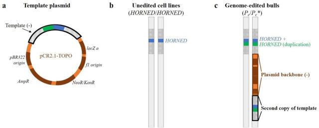
Here is what they claim happened (Fig 1): The template DNA is there, as evidenced by the PCR genotyping, but it inserted twice, with the rest of the plasmid in-between.

F1.large-5.jpg

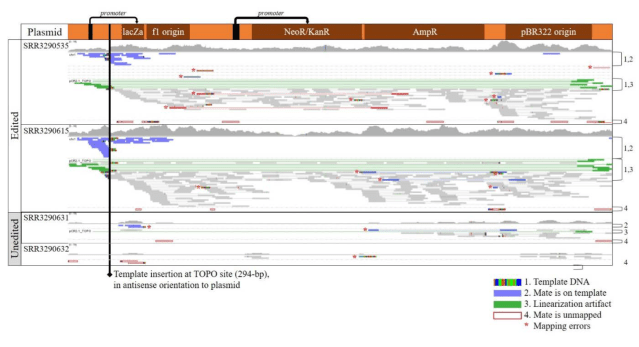
Here is the evidence (Supplementary figs 1 and 2): These are two annotated screenshots from IGV. The first shows alignments of reads from the calves and the unedited cell lines to the plasmid sequence. In the unedited cells, there are only stray reads, probably misplaced, but in the edited calves, ther are reads covering the plasmid throughout. Unless somehow else contaminated, this shows that the plasmid is somewhere in their genomes.

igv.png

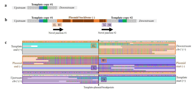
Where is it then? This second supplementary figure shows alignments to expected junctions: where template DNA and genome are supposed to join. The colourful letters are mismatches, showing where unexpected DNA shows up. This is the evidence for where the plasmid integrated and what kind of complex rearrangement of template, plasmid and genome happened at the cut site. This must have been found by looking at alignments, hypothesising an insertion, and looking for the junctions supporting it.

igv2.png

Why didn’t the PCR and targeted sequencing find this? As this third supplementary figure shows, the PCRs used could, theoretically, produce longer products including plasmid sequence. But they are way too long for regular PCR.

pcr.png

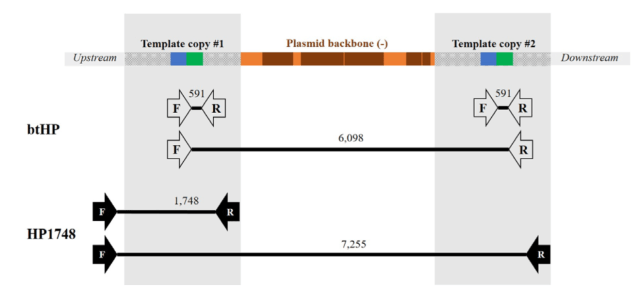
Looking at this picture, I wonder if there were a few attempts to make a primer pair that went from insert into the downstream sequence, that failed and got blamed on bad primer design or PCR conditions.

In summary, the 2019 preprint finds indirect evidence of the plasmid insertion by looking hard at short read alignments. Targeted sequencing or long read sequencing could give better evidence by observing he whole insertion. Recombinetics have acknowledged the problem, which makes me think that they’ve gone back to the DNA samples and checked.

Where does that leave us with quality control of gene editing? There are three kinds of problems to worry about:

  • Off-target edits in similar places in other parts of the genome; this seems to be what people used to worry about the most, and what Carlson & al checked for
  • Complex rearrangements around cut site (probably due to repeated cutting; this became a big concern after Kosicki & al (2018), and should apply both to on- and off-target cuts
  • Insertion of plasmid or mutated target; this is what happened in here

The ways people check gene edits (targeted Sanger sequencing and short read sequencing) doesn’t detect any of them particularly well, at least not without bespoke analysis. Maybe the kind of analysis that Norris & al do could be automated to some extent, but currently, the state of the art seems to be to manually look closely at alignments. If I was reviewing the preprint, I would have liked it if the manuscript had given a fuller description of how they arrived at this picture, and exactly what the evidence for this particular complex rearrangement is. This is a bit hard to follow.

Finally, is this embarrassing? On the one hand, this is important stuff, plasmid integration is a known problem, so the original researchers probably should have looked harder for it. On the other hand, the cell lines were edited and the clones born before a lot of the discussion and research of off-target edits and on-target rearrangements that came out of CRISPR being widely applied, and when long read sequencing was a lot less common. Maybe it was easier to think that the sort read off-target analysis was enough then. In any case, we need a solid way to quality check edits.

Literature

Molteni M. (2019) Brazil’s plan for gene edited-cows got scrapped–here’s why. Wired.

Carlson DF, et al. (2016) Production of hornless dairy cattle from genome-edited cell lines. Nature Biotechnology.

Norris AL, et al. (2019) Template plasmid integration in germline genome-edited cattle. BioRxiv.

Tan W, et al. (2013) Efficient nonmeiotic allele introgression in livestock using custom endonucleases. Proceedings of the National Academy of Sciences.

Bastiaansen JWM, et al. (2018) The impact of genome editing on the introduction of monogenic traits in livestock. Genetics Selection Evolution.

Kosicki M, Tomberg K & Bradley A. (2018) Repair of double-strand breaks induced by CRISPR–Cas9 leads to large deletions and complex rearrangements. Nature Biotechnology.

Temple Grandin at Roslin: optimisation and overselection

A couple of months ago (16 May to be precise), I listened to a talk by Temple Grandin at the Roslin Institute.

Grandin is a captivating speaker, and as an animal scientist (of some kind), I’m happy to have heard her talk at least once. The lecture contained a mix of:

  • practical experiences from a career of troubleshooting livestock management and systems,
  • how thinking differently (visually) helps in working with animal behaviour,
  • terrific personal anecdotes, among other things about starting up her business as a livestock management consultant from a student room,
  • a recurring theme, throughout the talk, of unintended side-effects in animal breeding, framed as a risk of ”overselecting” for any one trait, uncertainty about ”what is optimal”, and the importance of measuring and soberly evaluating many different things about animals and systems.

This latter point interests me, because it concerns genetics and animal breeding. Judging by the question in the Q&A, it also especially interested rest of the audience, mostly composed of vet students.

Grandin repeatedly cautioned against ”overselecting”. She argued that if you take one trait, any trait, and apply strong directional selection, bad side-effects will emerge. As a loosely worded biological principle, and taken to extremes, this seems likely to be true. If we assume that traits are polygenic, that means both that variants are likely to be pleiotropic (because there are many causal variants and a limited number of genes; this one argument for the omnigenic model) and that variants are likely to be linked to other variants that affect other traits. So changing one trait a lot is likely to affect other traits. And if we assume that the animal was in a pretty well-functioning state before selection, we should expect that if some trait that we’re not consciously selecting on changes far enough from that state, that is likely to cause problems.

We can also safely assume that there are always more traits that we care about than we can actually measure, either because they haven’t become a problem yet, or because we don’t have a good way to measure them. Taken together, this sound like a case for being cautious, measuring a lot of things about animal performance and welfare, and continuously re-evaluating what one is doing. Grandin emphasised the importance of measurement, drumming in that: ”you will manage what you measure”, ”this happens gradually”, and therefore, there is a risk that ”the bad becomes the new normal” if one does not keep tabs on the situation by recording hard quantitative data.

Doesn’t this sound a lot like the conventional view of mainstream animal breeding? I guess it depends: breeding is a big field, covering a lot of experiences and views, from individual farmers’ decisions, through private and public breeding organisations, to the relative Castalia of academic research. However, the impression from my view of the field, is Grandin and mainstream animal breeders are in agreement about the importance of:

  1. recording lots of traits about all aspects of the performance and functioning of the animal,
  2. optimising them with good performance on the farm as the goal,
  3. constantly re-evaluating practice and updating the breeding goals and management to keep everything on track.

To me, what Grandin presented as if it was a radical message (and maybe it was, some time ago, or maybe it still is, in some places) sounded much like singing the praises of economic selection indices. I had expected something more controversial. Then again, that depends on what assumptions are built into words like ”good performance”, ”on track”, ”functioning of the animal” etc. For example, she talked a bit about the strand of animal welfare research that aims to quantify positive emotions in animals; one could take the radical stance that we should measure positive emotions and include that in the breeding goal.

”Overselection” as a term also carries connotations that I don’t agree with, because I don’t think that the framing as biological overload is helpful. To talk about overload and ”overselection” makes one think of selection as a force that strains the animal in itself, and the alternative as ”backing off” (an expression term Grandin repeatedly used in the talk). But if the breeding goal is off the mark, in the sense that it doesn’t get towards what’s actually optimal for the animal on the farm, breeding less efficiently is not getting you to a better outcome; it only gets towards the same, suboptimal, outcome more slowly. The problem isn’t efficiency in itself, but misspecification, and uncertainty about what the goal should be.

Grandin expands on this idea in the introductory chapter to ”Are we pushing animals to their biological limits? Welfare and ethical applications” (Grandin & Whiting 2018, eds). (I don’t know much about the pig case used as illustration, but I can think of a couple of other examples that illustrate the same point.) It ends with this great metaphor about genomic power tools, that I will borrow for later:

We must be careful not to repeat the mistakes that were made with conventional breeding where bad traits were linked with desirable traits. One of the best ways to prevent this is for both animal and plant breeders to do what I did in the 1980s and 1990s: I observed many different pigs from many places and the behaviour problems became obvious. This enabled me to compare animals from different lines in the same environment. Today, both animal and plant breeders have ‘genomic power tools’ for changing an organism’s genetics. Power tools are good things, but they must be used carefully because changes gan be made more quickly. A circular saw can chop your hand off much more easily than a hand saw. It has to be used with more care.

Jennifer Doudna & Samuel Sternberg ”A Crack In Creation”

While the blog is on a relaxed summer schedule, you can read my book review of Jennifer Doudna’s and Samuel Sternberg’s CRISPR-related autobiography and discussion of the future of genome editing in University of Edinburgh’s Science Magazine EUSci issue #24.

The book is called A Crack in Creation, subtitled The New Power to Control Evolution, or depending on edition, Gene Editing and the Unthinkable Power to Control Evolution. There are a couple of dramatic titles for you. The book starts out similarly dramatic, with Jennifer Doudna dreaming of a beach in Hawaii, where she comes from, imagining a wave rising from the ocean to crash down on her. The wave is CRISPR/Cas9 genome editing, the technological force of nature that Doudna and colleagues have let loose on the world.

I like the book, talk about some notable omissions, and take issue with the bombastic and inaccurate title(s). Read the rest here.

Links

Pivotal CRISPR patent battle won by Broad Institute. Nature News. 2018.

Sharon Begley & Andrew Joseph. The CRISPR shocker: How genome-editing scientist He Jiankui rose from obscurity to stun the world. Stat News. 2018.

A Crack in Creation. The book’s website.

‘Simulating genetic data with R: an example with deleterious variants (and a pun)’

A few weeks ago, I gave a talk at the Edinburgh R users group EdinbR on the RAGE paper. Since this is an R meetup, the talk concentrated on the mechanics of genetic data simulation and with the paper as a case study. I showed off some of what Chris Gaynor’s AlphaSimR can do, and how we built on that to make the specifics of this simulation study. The slides are on the EdinbR Github.

Genetic simulation is useful for all kinds of things. Sure, they’re only as good as the theory that underpins them, but the willingness to try things out in simulations is one of the things I always liked about breeding research.

This is my description of the logic of genetic simulation: we think of the genome as a large table of genotypes, drawn from some distribution of allele frequencies.

To make an utterly minimal simulation, we could draw allele frequencies from some distribution (like a Beta distribution), and then draw the genotypes from a binomial distribution. Done!

However, there is a ton of nuance we would like to have: chromosomes, linkage between variants, sexes, mating, selection …

AlphaSimR addresses all of this, and allows you to throw individuals and populations around to build pretty complicated designs. Here is the small example simulation I used in the talk.


library(AlphaSimR)
library(ggplot2)

## Generate founder chromsomes

FOUNDERPOP <- runMacs(nInd = 1000,
                      nChr = 10,
                      segSites = 5000,
                      inbred = FALSE,
                      species = "GENERIC")


## Simulation parameters

SIMPARAM <- SimParam$new(FOUNDERPOP)
SIMPARAM$addTraitA(nQtlPerChr = 100,
                   mean = 100,
                   var = 10)
SIMPARAM$addSnpChip(nSnpPerChr = 1000)
SIMPARAM$setGender("yes_sys")


## Founding population

pop <- newPop(FOUNDERPOP,
              simParam = SIMPARAM)

pop <- setPheno(pop,
                varE = 20,
                simParam = SIMPARAM)


## Breeding

print("Breeding")
breeding <- vector(length = 11, mode = "list")
breeding[[1]] <- pop

for (i in 2:11) {
    print(i)
    sires <- selectInd(pop = breeding[[i - 1]],
                       gender = "M",
                       nInd = 25,
                       trait = 1,
                       use = "pheno",
                       simParam = SIMPARAM)

    dams <- selectInd(pop = breeding[[i - 1]],
                      nInd = 500,
                      gender = "F",
                      trait = 1,
                      use = "pheno",
                      simParam = SIMPARAM)

    breeding[[i]] <- randCross2(males = sires,
                                females = dams,
                                nCrosses = 500,
                                nProgeny = 10,
                                simParam = SIMPARAM)
    breeding[[i]] <- setPheno(breeding[[i]],
                              varE = 20,
                              simParam = SIMPARAM)
}


## Look at genetic gain and shift in causative variant allele frequency

mean_g <- unlist(lapply(breeding, meanG))
sd_g <- sqrt(unlist(lapply(breeding, varG)))

plot_gain <- qplot(x = 1:11,
                   y = mean_g,
                   ymin = mean_g - sd_g,
                   ymax = mean_g + sd_g,
                   geom = "pointrange",
                   main = "Genetic mean and standard deviation",
                   xlab = "Generation", ylab = "Genetic mean")

start_geno <- pullQtlGeno(breeding[[1]], simParam = SIMPARAM)
start_freq <- colSums(start_geno)/(2 * nrow(start_geno))

end_geno <- pullQtlGeno(breeding[[11]], simParam = SIMPARAM)
end_freq <- colSums(end_geno)/(2 * nrow(end_geno))

plot_freq_before <- qplot(start_freq, main = "Causative variant frequency before") 
plot_freq_after <- qplot(end_freq, main = "Causative variant frequency after") 

This code builds a small livestock population, breeds it for ten generations, and looks at the resulting selection response in the form of a shift of the genetic mean, and the changes in the underlying distribution of causative variants. Here are the resulting plots:

‘Approaches to genetics for livestock research’ at IASH, University of Edinburgh

A couple of weeks ago, I was at a symposium on the history of genetics in animal breeding at the Institute of Advanced Studies in the Humanities, organized by Cheryl Lancaster. There were talks by two geneticists and two historians, and ample time for discussion.

First geneticists:

Gregor Gorjanc presented the very essence of quantitative genetics: the pedigree-based model. He illustrated this with graphs (in the sense of edges and vertices) and by predicting his own breeding value for height from trait values, and from his personal genomics results.

Then, yours truly gave this talk: ‘Genomics in animal breeding from the perspectives of matrices and molecules’. Here are the slides (only slightly mangled by Slideshare). This is the talk I was preparing for when I collected the quotes I posted a couple of weeks ago.

I talked about how there are two perspectives on genomics: you can think of genomes either as large matrices of ancestry indicators (statistical perspective) or as long strings of bases (sequence perspective). Both are useful, and give animal breeders and breeding researchers different tools (genomic selection, reference genomes). I also talked about potential future breeding strategies that use causative variants, and how they’re not about stopping breeding and designing the perfect animal in a lab, but about supplementing genomic selection in different ways.

Then, historians:

Cheryl Lancaster told the story of how ABGRO, the Animal Breeding and Genetics Research Organisation in Edinburgh, lost its G. The organisation was split up in the 1950s, separating fundamental genetics research and animal breeding. She said that she had expected this split to be do to scientific, methodological or conceptual differences, but instead found when going through the archives, that it all was due to personal conflicts. She also got into how the ABGRO researchers justified their work, framing it as ”fundamental research”, and aspired to do long term research projects.

Jim Lowe talked about the pig genome sequencing and mapping efforts, how it was different from the human genome project in organisation, and how it used comparisons to the human genome a lot. Here he’s showing a photo of Alan Archibald using the gEVAL genome browser to quality-check the pig genome. He also argued that the infrastructural outcomes of a project like the human genome project, such as making it possible for pig genome scientists to use the human genome for comparisons, are more important and less predictable than usually assumed.

The discussion included comments by some of the people who were there (Chris Haley, Bill Hill), discussion about the breed concept, and what scientists can learn from history.

What is a breed? Is it a genetical thing, defined by grouping individuals based on their relatedness, a historical thing, based on what people think a certain kind of animal is supposed to look like, or a marketing tool, naming animals that come from a certain system? It is probably a bit of everything. (I talked with Jim Lowe during lunch; he had noticed how I referred to Griffith & Stotz for gene concepts, but omitted the ”post-genomic” gene concept they actually favour. This is because I didn’t find it useful for understanding how animal breeding researchers think. It is striking how comfortable biologists are with using fuzzy concepts that can’t be defined in a way that cover all corner cases, because biology doesn’t work that way. If the nominal gene concept is broken by trans-splicing, practicing genomicists will probably think of that more as a practical issue with designing gene databases than a something that invalidates talking about genes in principle.)

What would researchers like to learn from history? Probably how to succeed with large research endeavors and how to get funding for them. Can one learn that from history? Maybe not, but there might be lessons about thinking of research as ”basic”, ”fundamental”, ”applied” etc, and about what the long term effects of research might be.

What single step does with relationship

We had a journal club about the single step GBLUP method for genomic evaluation a few weeks ago. In this post, we’ll make a few graphs of how the single step method models relatedness between individuals.

Imagine you want to use genomic selection in a breeding program that already has a bunch of historical pedigree and trait information. You could use some so-called multistep evaluation that uses one model for the classical pedigree + trait quantitative genetics and one model for the genotype + trait genomic evaluation, and then mix the predictions from them together. Or you could use the single-step method, which combines pedigree, genotypes and traits into one model. It does this by combining the relationship estimates from pedigree and genotypes. That matrix can then go into your mixed model.

We’ll illustrate this with a tiny simulated population: five generations of 100 individuals per generation, where ten random pairings produce the next generation, with families of ten individuals. (The R code is on Github and uses AlphaSimR for simulation and AGHmatrix for matrices). Here is a heatmap of the pedigree-based additive relationship matrix for the population:

What do we see? In the lower left corner are the founders, and not knowing anything about their heritage, the matrix has them down as unrelated. The squares of high relatedness along the diagonal are the families in each generation. As we go upwards and to the right, relationship is building up.

Now, imagine the last generation of the population also has been genotyped with a SNP chip. Here is a heatmap of their genomic relationship matrix:

Genomic relationship is more detailed. We can still discern the ten families within the last generation, but no longer are all the siblings equally related to each other and to their ancestors. The genotyping helps track segregation within families, pointing out to us when relatives are more or less related than the average that we get from the pedigree.

Enter the single-step relationship matrix. The idea is to put in the genomic relationships for the genotyped individuals into the big pedigree-based relationship matrix, and then adjust the rest of the matrix to propagate that extra information we now have from the genotyped individuals to their ungenotyped relatives. Here is the resulting heatmap:

You can find the matrix equations in Legarra, Aguilar & Misztal (2009). The matrix, called H, is broken down into four partitions called H11, H12, H21, and H22. H22 is the part that pertains to the genotyped animals, and it’s equal to the genomic relationship matrix G (after some rescaling). The others are transformations of G and the corresponding parts of the additive relationship matrix, spreading G onto A.

To show what is going on, here is the difference between the additive relationship matrix and the single-step relationship matrix, with lines delineating the genotyped animals and breaking the matrix into the four partitions:

What do we see? In the top right corner, we have a lot of difference, where the genomic relationship matrix has been plugged in. Then, fading as we go from top to bottom and from right to left, we see the influence of the genomic relationship on relatives, diminishing the further we get from the genotyped individuals.

Literature

Legarra, Andres, I. Aguilar, and I. Misztal. ”A relationship matrix including full pedigree and genomic information.” Journal of dairy science 92.9 (2009): 4656-4663.

Excerpts about genomics in animal breeding

Here are some good quotes I’ve come across while working on something.

Artificial selection on the phenotypes of domesticated species has been practiced consciously or unconsciously for millennia, with dramatic results. Recently, advances in molecular genetic engineering have promised to revolutionize agricultural practices. There are, however, several reasons why molecular genetics can never replace traditional methods of agricultural improvement, but instead they should be integrated to obtain the maximum improvement in economic value of domesticated populations.

Lande R & Thompson R (1990) Efficiency of marker-assisted selection in the improvement of quantitative traits. Genetics.

Smith and Smith suggested that the way to proceed is to map QTL to low resolution using standard mapping methods and then to increase the resolution of the map in these regions in order to locate more closely linked markers. In fact, future developments should make this approach unnecessary and make possible high resolution maps of the whole genome, even, perhaps, to the level of the DNA sequence. In addition to easing the application of selection on loci with appreciable individual effects, we argue further that the level of genomic information available will have an impact on infinitesimal models. Relationship information derived from marker information will replace the standard relationship matrix; thus, the average relationship coefficients that this represents will be replaced by actual relationships. Ultimately, we can envisage that current models combining few selected QTL with selection on polygenic or infinitesimal effects will be replaced with a unified model in which different regions of the genome are given weights appropriate to the variance they explain.

Haley C & Visscher P. (1998) Strategies to utilize marker–quantitative trait loci associations. Journal of Dairy Science.

Instead, since the late 1990s, DNA marker genotypes were included into the conventional BLUP analyses following Fernando and Grossman (1989): add the marker genotype (0, 1, or 2, for an animal) as a fixed effect to the statistical model for a trait, obtain the BLUP solutions for the additive polygenic effect as before, and also obtain the properly adjusted BLUE solution for the marker’s allele substitution effect; multiply this BLUE by 0, 1, or 2 (specic for the animal) and add the result to the animal’s BLUP to obtain its marker-enhanced EBV. A logical next step was to treat the marker genotypes as semi-random effects, making use of several different shrinkage strategies all based on the marker heritability (e.g., Tsuruta et al., 2001); by 2007, breeding value estimation packages such as PEST (Neumaier and Groeneveld, 1998) supported this strategy as part of their internal calculations. At that time, a typical genetic evaluation run for a production trait would involve up to 30 markers.

Knol EF, Nielsen B, Knap PW. (2016) Genomic selection in commercial pig breeding. Animal Frontiers.

Although it has not caught the media and public imagination as much as transgenics and cloning, genomics will, I believe, have just as great a long-term impact. Because of the availability of information from genetically well-researched species (humans and mice), genomics in farm animals has been established in an atypical way. We can now see it as progressing in four phases: (i) making a broad sweep map (~20 cM) with both highly informative (microsatellite) and evolutionary conserved (gene) markers; (ii) using the informative markers to identify regions of chromosomes containing quantitative trait loci (QTL) controlling commercially important traits–this requires complex pedigrees or crosses between phenotypically anc genetically divergent strains; (iii) progressing from the informative markers into the QTL and identifying trait genes(s) themselves either by complex pedigrees or back-crossing experiments, and/or using the conserved markers to identify candidate genes from their position in the gene-rich species; (iv) functional analysis of the trait genes to link the genome through physiology to the trait–the ‘phenotype gap’.

Bulfield G. (2000) Biotechnology: advances and impact. Journal of the Science of Food and Agriculture.

I believe animal breeding in the post-genomic era will be dramatically different to what it is today. There will be massive research effort to discover the function of genes including the effect of DNA polymorphisms on phenotype. Breeding programmes will utilize a large number of DNA-based tests for specific genes combined with new reproductive techniques and transgenes to increase the rate of genetic improvement and to produce for, or allocate animals to, the product line to which they are best suited. However, this stage will not be reached for some years by which time many of the early investors will have given up, disappointed with the early benefits.

Goddard M. (2003). Animal breeding in the (post-) genomic era. Animal Science.

Genetics is a quantitative subject. It deals with ratios, with measurements, and with the geometrical relationships of chromosomes. Unlike most sciences that are based largely on mathematical techniques, it makes use of its own system of units. Physics, chemistry, astronomy, and physiology all deal with atoms, molecules, electrons, centimeters, seconds, grams–their measuring systems are all reducible to these common units. Genetics has none of these as a recognizable component in its fundamental units, yet it is a mathematically formulated subject that is logically complete and self-contained.

Sturtevant AH & Beadle GW. (1939) An introduction to genetics. W.B. Saunders company, Philadelphia & London.

We begin by asking why genes on nonhomologous chromosomes assort independently. The simple cytological story rehearsed above answers the questions. That story generates further questions. For example, we might ask why nonhomologous chromosomes are distributed independently at meiosis. To answer this question we could describe the formation of the spindle and the migration of chromosomes to the poles of the spindle just before meiotic division. Once again, the narrative would generate yet further questions. Why do the chromosomes ”condense” at prophase? How is the spindle formed? Perhaps in answering these questions we would begin to introduce the chemical details of the process. Yet simply plugging a molecular account into the narratives offered at the previous stages would decrease the explanatory power of those narratives.

Kitcher, P. (1984) 1953 and all that. A tale of two sciences. Philosophical Review.

And, of course, this great quote by Jay Lush.

There is no breeder’s equation for environmental change

This post is about why heritability coefficients of human traits can’t tell us what to do. Yes, it is pretty much an elaborate subtweet.

Let us begin in a different place, where heritability coefficients are useful, if only a little. Imagine there is selection going on. It can be natural or artificial, but it’s selection the old-fashioned way: there is some trait of an individual that makes it more or less likely to successfully reproduce. We’re looking at one generation of selection: there is one parent generation, some of which reproduce and give rise to the offspring generation.

Then, if we have a well-behaved quantitative trait, no systematic difference between the environments that the two generations experience (also, no previous selection; this is one reason I said ‘if only a little’), we can get an estimate of the response to selection, that is how the mean of the trait will change between the generations:

R = h^2S

R is the response. S, the selection differential, is the difference between the mean all of the parental generation and the selected parents, and thus measures the strength of the selection. h2 is the infamous heritability, which measures the accuracy of the selection.

That is, the heritability coefficient tells you how well the selection of parents reflect the offspring traits. A heritability coefficient of 1 would mean that selection is perfect; you can just look at the parental individuals, pick the ones you like, and get the whole selection differential as a response. A heritability coefficient of 0 means that looking at the parents tells you nothing about what their offspring will be like, and selection thus does nothing.

Conceptually, the power of the breeder’s equation comes from the mathematical properties of selection, and the quantitative genetic assumptions of a linear parent–offspring relationship. (If you’re a true connoisseur of theoretical genetics or a glutton for punishment, you can derive it from the Price equation; see Walsh & Lynch (2018).) It allows you to look (one generation at a time) into the future only because we understand what selection does and assume reasonable things about inheritance.

We don’t have that kind machinery for environmental change.

Now, another way to phrase the meaning of the heritability coefficient is that it is a ratio of variances, namely the additive genetic variance (which measures the trait variation that runs in families) divided by the total variance (which measures the total variation in the population, duh). This is equally valid, more confusing, and also more relevant when we’re talking about something like a population of humans, where no breeding program is going on.

Thus, the heritability coefficient is telling us, in a specific highly geeky sense, how much of trait variation is due to inheritance. Anything we can measure about a population will have a heritability coefficient associated with it. What does this tell us? Say, if drug-related crime has yay big heritability, does that tell us anything about preventing drug-related crime? If heritability is high, does that mean interventions are useless?

The answers should be evident from the way I phrased those rhetorical questions and from the above discussion: There is no theoretical genetics machinery that allows us to predict the future if the environment changes. We are not doing selection on environments, so the mathematics of selection don’t help us. Environments are not inherited according to the rules of quantitative genetics. Nothing prevents a trait from being eminently heritable and respond even stronger to changes in the environment, or vice versa.

(There is also the argument that quantitative genetic modelling of human traits matters because it helps control for genetic differences when estimating other factors. One has to be more sympathetic towards that, because who can argue against accurate measurement? But ought implies can. For quantitative genetic models to be better, they need to solve the problems of identifying variance components and overcoming population stratification.)

Much criticism of heritability in humans concern estimation problems. These criticisms may be valid (estimation is hard) or silly (of course, lots of human traits have substantial heritabilities), but I think they miss the point. Even if accurately estimated, heritabilities don’t do us much good. They don’t help us with the genetic component, because we’re not doing breeding. They don’t help us with the environmental component, because there is no breeder’s equation for environmental change.

Paper: ‘Removal of alleles by genome editing (RAGE) against deleterious load’

Our new paper is about using predicted deleterious variants in animal breeding. We use simulation to look at the potential to improve livestock fitness by either selecting on detected deleterious variants or removing deleterious alleles by genome editing.

Summary

Deleterious variants occur when errors in DNA replication that disrupt the function of a gene. Such errors are frequent enough that all organisms carry mildly deleterious variants. Geneticists describe this as a deleterious load, that cause organisms to be less healthy and fit than they could have been if these errors didn’t happen. Load is especially pertinent to livestock populations, because of their relatively small population sizes and inbreeding.

Historically, it has not been possible to observe deleterious variants directly, but as genome sequencing becomes cheaper and new bioinformatic methods are being developed, we can now sequence livestock and detect variants that are likely to be deleterious.

In this study, we used computer simulation to see how future breeding strategies involving selection or genome editing could be used to reduce deleterious load. We tested selection against deleterious load and genome editing strategy we call RAGE (Removal of Alleles by Genome Editing) in simulated livestock populations to see how it improved fitness. The simulations suggest that selecting on deleterious variants identified from genome sequencing may help improve fitness of livestock populations, and that genome editing to remove deleterious variants could improve them even more.

For these strategies to be effective, it is important that detection of deleterious variants is accurate, and genome editing of more than one variant per animal would need to become possible without damaging side-effects. Future research on how to measure deleterious load in large sequence datasets from livestock animals, and how to perform genome editing safely and effectively will be important.

Figure 2 from the paper, showing the average fitness of simulated populations (y-axis) over the generations of breeding (x-axis) with different types of future breeding against deleterious variants.

‘RAGE against …’, what’s with the acronym?

We are very happy with the acronym. In addition to making at least two pop culture references, it’s also a nod to Promotion of Alleles by Genome Editing (PAGE) from Jenko et al. (2015). I like that the acronyms, both PAGE and RAGE, emphasises that we’re dealing with alleles that already exist within a population. We propose using genome editing as a way to promote alleles we like and remove alleles we don’t like in addition to classical breeding. The fancy new biotechnology does not replace selection, but supplements it.

Do you really think one should genome edit farm animals?

Yes, if all the bio- and reproductive technology can be made to work! Currently, genome editing methods like Crispr/Cas9 require many attempts to get precise editing to the desired allele at one place, and it doesn’t scale to multiple edits in the same animal … Not yet. But lots of smart people are competing to make it happen.

Genome editing of farm animals would also need a lot of reproductive technology, that currently isn’t really there (but probably more so for cattle than for other species). Again, lots of clever people work on it.

If it can be made to work, genome editing could be a useful breeding method.

What about the ethics of genome editing?

We don’t discuss ethics much in the paper. In one simple sense, that is because ethics isn’t our expertise. I also think a discussion of the ethics of RAGE, much like an informed discussion about the economics of it, requires empirical knowledge that we don’t have yet.

I am not of the opinion that there is a dignity or integrity to the genome that would prohibit genome editing as a rule. So the question is not ‘genome editing or not’, but ‘under what circumstances and for what applications is genome editing useful and justified?’ and ‘are the benefits of RAGE, PAGE, or whatever -GE, enough to outweigh the risks and costs?’. There is room for uncertainty and disagreement about those questions.

For a good discussion of the ethics of genome editing that is likely to raise more questions than it answers, see Eriksson et al. (2018). Among other things, they make the point that advanced reproductive technologies is a precondition for genome editing, but kind of slips out of the discussion sometimes. I think the most pressing question, both from the ethical and economical perspective, is whether the benefits of genome editing are enough to justify widespread use of reproductive technologies (in species where that isn’t already commonplace). I also like how they make the point that one needs to look at the specific applications of genome editing, in context, when evaluating them.

The simulation looks nifty! I want to simulate breeding programs like that!

You can! The simulations used the quantitative genetic simulation R package AlphaSimR with some modifications for simulating the fitness traits. There is code with the paper. Here are also the slides from when I talked about the paper at the Edinburgh R user group.

You make a ton of assumptions!

We do. Some of them are extremely uncontroversial (the basic framework of segregation and recombination during inheritance), some we can get some idea about by looking at the population genetics literature (we’ve taken inspiration from estimates of deleterious mutation rates and effect distributions estimated from humans), and some we don’t have much knowledge about at all (how does load of deleterious variants relate to the production, reproduction and health traits that are important to breeding? The only way to know is to measure). If you read the paper, don’t skip that part of the Discussion.

Would this work in plants?

Yes, probably! Plant breeding programs are a bit different, so I guess one should simulate them to really know. RAGE would be a part of the ‘Breeding 4.0’ logic of Wallace, Rodgers-Melnick & Butler (2018). In many ways the problems with plants are smaller, with less unknown reproductive technology that needs to be invented first, and an easier time field testing edited individuals.

Literature

Johnsson M, Gaynor RC, Jenko J, Gorjanc G, de Koning D-J, Hickey, JM. (2019) Removal of alleles by genome editing (RAGE) against deleterious load. Genetics Selection Evolution.

Jenko J, Gorjanc G, Cleveland MA, Varshney RK, Whitelaw CBA, Woolliams JA, Hickey JM. (2015). Potential of promotion of alleles by genome editing to improve quantitative traits in livestock breeding programs. Genetics Selection Evolution.

Eriksson, S., Jonas, E., Rydhmer, L., & Röcklinsberg, H. (2018). Invited review: Breeding and ethical perspectives on genetically modified and genome edited cattle. Journal of dairy science, 101(1), 1-17.

Wallace, J. G., Rodgers-Melnick, E., & Buckler, E. S. (2018). On the road to Breeding 4.0: unraveling the good, the bad, and the boring of crop quantitative genomics. Annual review of genetics, 52, 421-444.

‘Any distinction in principle between qualitative and quantitative characters disappeared long ago’

Any distinction in principle between qualitative and quantitative characters disappeared long ago, although in the early days of Mendelism it was often conjectured that they might be inherited according to fundamentally different laws.

If it is still convenient to call some characters qualitative and others quantitative, it is only to denote that the former naturally have a discontinuous and the latter a continuous distribution, or that the former are not easily measured on a familiar metrical scale. Colors are an example. Differences between colors can be measured in terms of length of light waves, hue, brilliance etc., but most of us find it difficult to compare those measurements with our own visual impressions.

Most quantitative characters are affected by many pairs of genes and also importantly by environmental variations. It is rarely possible to identify the pertinent genes in a Mendelian way or to map the chromosomal position of any of them. Fortunately this inability to identify and describe the genes individually is almost no handicap to the breeder of economic plants or animals. What he would actually do if he knew the details about all the genes which affect a quantitative character in that population differs little from what he will do if he merely knows how heritable it is and whether much of the hereditary variance comes from dominance or overdominance, and from epistatic interactions between the genes.

(That last part might not always be true anymore, but it still remained on point for more than half the time that genetics as a discipline has existed.)

Jay L Lush (1949) Heritability of quantitative characters in farm animals