Den ökända krigargenen möter Vetenskapens värld

SVT:s Vetenskapens värld sände nyligen (17 oktober, ”Ditt förutbestämda liv”) ett program om beteendegenetik. Det handlar om en studie i Dunedin, Nya Zeeland, som kopplar varianter av vissa gener, i kombination med påfrestande händelser under livets gång, till antisocialt beteende, depression med mera. SVT och dokumentären presenterar den som ”en oerhörd studie” som ”skrivit om den klassiska frågan om arv och miljö och visat att kombinationen är det avgörande”. Men det är snarare en stilstudie i hur välmenande forskare kan ha otur, dra förhastade slutsatser och skapa ett nystan av överdrifter. Otur och otur, förresten, för dem själva ledde det ju till berömmelse och dokumentärer som når ända till Sverige. Men för vetenskapen om den genetiska grunden för beteende var det ändå mest otur.

På 00-talet, när studierna ifråga publicerades, var beteendegenetiker väldigt optimistiska om vad som krävdes för att hitta gener som förklarar komplexa egenskaper, till exempel våldsamt beteende, depression med mera. Många trodde att det räckte att göra som i Dunedin, samla in data från kanske 1000 individer och välja ut en gen, en så kallad ”kandidatgen”, att studera. Komplexa egenskaper, som mänskligt beteende, kan visst ha en avsevärd ärftlig komponent. Men den består av hundratals, kanske tusentals, okända genetiska varianter med små effekter. Dagens genetik har gått vidare till att studera tiotusentals eller hundratusentals individer för att ha en chans att hitta några varianter, och till att studera alla gener samtidigt istället för att försöka gissa vilka kandidatgener som är viktiga.

Men tusen människor, hör jag er protestera, det är väl ändå många? I fallet MAOA tittar de bara på män, så där ryker hälften. Sedan är det ungefär en tredjedel av dem som har riskvarianten, och en bråkdel av dem som haft en dålig uppväxt. I dokumentären låter kopplingen mellan MAOA, dålig uppväxt och antisocialt beteende så övertygande. Richie Poulton, en av författarna, säger: ”Om man tittar på de killar som har riskvarianten av genen och som blev gravt illa behandlade, så uppvisade hela 85% av dem någon form av antisocialt beteende när de blivit vuxna [min översättning].” I själva verket, om man läser artikeln, så består gruppen han talar om – män med riskvarianten som blivit gravt illa behandlade under uppväxten – av 13 individer. De 85% han talar om är alltså elva män. Hur många av dem hade, enligt originalartikeln dömts för något våldsbrott vid 26 års ålder? Svaret är fyra. Med ett stickprov på 13 människor får man inga bra mått på vad riskvarianten har för effekt. Man får brus.

Och brus är precis vad som kommer ur kandidatgenstudier inom psykiatrisk genetik. Det går till ungefär så här: Någon hittar en kandidatgen i en liten studie, dåförtiden med stor buller och bång. Sedan kommer dussintals liknande studier med motsägelsefulla resultat. Ibland hittar de något liknande, ibland inte. Ibland hittar de en effekt på något annat: en interaktion med något nytt, en annan vagt relaterad egenskap. Efter hand börjar folk göra meta-analyser, som lägger ihop resultaten från många studier. De visar på stor variation och små effekter. Och så går det vidare. När det till slut börjar komma studier med större urval, som tittar på hela arvsmassan, så syns det (med några lysande undantag som apolipoprotein E) oftast inte ett spår av kandidatgenerna.

Men visst, ingen har tittat efter varianter i hela genomet med just de gen–miljöinteraktioner som var i Dunedinstudien. Och associationsstudier av hela genomet har hittills bara hittat varianter som kan förklara en bråkdel av den genetiska variationen. Så de gamla kandidatgensfavoriterna kanske också gömmer sig där ute, även om det inte ser ut så. Oavsett är det klart att de inte kan vara mer än en bråkdel av förklaringen, och att metoden att gissa kandidatgener och testa dem i små stickprov inte fungerar något vidare. Men på teve och i pressmeddelanden finns det aldrig komplikationer eller negativa resultat. Därför är MAOA också känd som ”the warrior gene”. Den är ett perfekt provokativt exempel att ta upp när man vill säga att människor är stenhårt programmerade av evolutionen att bete sig på ett visst sätt. Eller, som i den här dokumentären, när man vill komma ett mer humanistiskt budskap om hur uppväxten kan övervinna generna.

Författarna och dokumentärmakarna har såklart rätt i att både arv och miljö spelar roll för komplexa egenskaper. De har kanske till och med rätt att gen–miljöinteraktioner, där effekten av en viss genetisk variant bara visar sig under speciella miljöförhållanden, är viktiga. Men de har fel i att varianter i MAOA spelar en avgörande roll. Om MAOA-varianten har någon effekt alls, vilket inte ens är säkert, så är den bara en variant med liten effekt bland hundratals andra. Resultat som MAOA-associationen i Dunedin är inte några genombrott som skakar beteendegenetiken i grunden. De är ärliga misstag från en ung vetenskap som för 15 år sedan ännu inte hade lärt sig hur svårt det är att hitta gener som förklarar komplexa egenskaper. Istället för att älta dem är det dags att lämna kandidatgenerna bakom sig och gå vidare.

(Det här inlägget är lite försenat, för jag försökte få en kortare version av den här texten publicerad. Jag vet inte vad jag tänkte där. SVT Vetenskap har inte heller svarat. Den som läste den blev väl stött, eller avskrev den ungefär som en arg insändare. Nåja. Efter själva programmet var det ett par svenska forskare som fick vara med och prata lite. De var nog bra på sina ämnen, men ingen av dem verkade veta särskilt mycket om genetik, och sa inget kritiskt om själva innehållet. Ingen kritiserade heller det orimliga skrytet som dokumentären var full av. Jag förstår att jag framstår som en surgubbe nu, men det kan inte hjälpas.)

Litteratur

Caspi et al. (2002) ”Role of genotype in the cycle of violence in maltreated children.” Science

Caspi et al. (2003) ”Influence of life stress on depression: moderation by a polymorphism in the 5-HTT gene.” Science.

Paper: ”Feralisation targets different genomic loci to domestication in the chicken”

It is out: Feralisation targets different genomic loci to domestication in the chicken. This is the second of our papers on the Kauai feral and admixed chicken population, and came out a few days ago.

The Kauai chicken population is kind of famous: you can find them for instance on Flickr, or on YouTube. We’ve previously looked at their plumage, listened to the roosters’ crowings, and sequenced mitochondrial DNA to investigate their origins. Based on this, we concur with the common view that the chickens of Kauai probably are a mixture of feral birds of domestic origin and wild Junglefowl. The Kauai chickens look and sound like a mix of wild and domestic, and we found mitochondrial DNA of two haplogroups, one of which (called D) is typical in ancient chicken DNA from Pacific islands (Gering et al 2015).

In this paper, we looked at the rest of the genome of the same chickens — you didn’t think we sequenced the whole thing just to look at the mitochondrion plus a subset of markers, did you? We turn to population genomics, and a family of methods called selective sweep mapping, to search for regions of their genome that show signs of being affected by natural selection. This lets us: 1) draw pretty rainbow plots such as  this one …

kauai2_fig1a

(Figure 1a from the paper in question, Johnsson & al 2016. cc:by The chromosomes have been laid out on the horizontal axis with different colours, and split into windows of 40 kb. Each dot represents the heterozygosity of that windows. For all the details, see the paper.)

… 2) highlight a regions of the genome that may have been selected during feralisation on Kauai (these are the icicles in the graph, highligthed by arrows); 3) conclude that the regions that look like they’ve been selected in feralisation overlap very little with the ones that look like they’ve been selected in chicken domestication. Hence the title.

That was the main result, but of course we also look at what genes are highlighted. Mostly we have no idea how they may contribute to feralisation, but a couple of regions overlap with those that we’ve previously found in genetic mapping of comb size and egg laying in our wild-by-domestic intercross. We also compare the potentially selected regions to domestic chicken sequences.

Last year, Ewen Callaway visited Dominic Wright, Eben Gering and Rie Henriksen on the last fieldtrip to Kauai. The article, When chickens go wild, was published in Nature News in January, and it explains a lot of the ideas nicely. This paper was submitted by then, so the samples they gathered on that trip do not feature in it. But, spoiler alert: there is more to come. (I don’t know what role I personally will play, but that is less important.)

As you may have guessed if you looked at the author list, this was a collaboration between quite a lot of people in Linköping, Michigan, London, and Victoria. Thanks to all involved! This was great fun, and for those of you who like this sort of thing, I hope the paper will be an interesting read.

Literature

M. Johnsson, E. Gering, P. Willis, S. Lopez, L. Van Dorp, G. Hellenthal, R. Henriksen, U. Friberg & D. Wright. (2016) Feralisation targets different genomic loci to domestication in the chicken. Nature Communications. doi:10.1038/ncomms12950

På dna-dagen: Genetik utan dna

Så här på dna-dagen tänkte jag skriva lite om vad som går att göra utan att veta något om dna, och varför det (förstås) blir ännu bättre med dna.

Vi tänker oss tillbaka till tiden före genomprojekt, sekvenseringsmaskiner och kloning. Säg någon gång i 1900-talets början. Vad vet vi om ärftlighet? Vi vet att egenskaper går i arv. Det behöver man inte vara något ljushuvud för att lägga märke till. Vi vet att djuravel och växtförädling fungerar. Det vill säga, om man väljer ut de individer som har egenskaper vi behöver och låter dem para sig, så kommer nästa generation bli ännu bättre. Det är 1700-talskunskap allra minst, och förmodligen mycket äldre än så. Vi har en teori om ärftlighet, från Mendel och hans berömda ärtor  Vi vet att ärftligheten består av anlag som blandas om varje generation, men utan att spädas ut. Det är de som idag kallas genetiska varianter.

Varje individ har en uppsättning genetiska varianter. De påverkar individens egenskaper, och de går vidare till nästa generation när individen får barn. Modernt uttryckt: Alla individer har gener, och de finns i olika genetiska varianter. Alla har två varianter av varje gen, och en av dem kommer gå vidare till varje avkomma. Vi vet ännu inte vad generna består av (spoiler: det är dna).

En del egenskaper är enkla, och verkar styras av varianter av en enda gen. En höna kan ha vita fjädrar eller färgade, till exempel; det styrs av varianter av en enda gen. Den ena varianten gör hönan vita fjädrar, och den andra tillåter andra färger att komma fram. Egenskapen delar in höns i två typer: vita höns och höns med andra färger.

Men de flesta egenskaper är inte så enkla. Ta hur mycket hönan väger. Höns kommer i alla storlekar, små, stora och mittemellan. Det är ofta sådana egenskaper som är viktigast. Hur stor blir hönan? Hur många ägg lägger hon? Hur rädd är hon för människor? Och så vidare. Hur gör vi om vi vill förstå en sådan kvantitativ egenskap?

Vi utgår ifrån det faktum att det finns många gener som påverkar en kvantitativ egenskap. Varje gen finns i flera varianter, och varje individ har två varianter. Vi börjar med att anta något helt orealistiskt, nämligen att vi vet exakt vilka genetiska varianter som finns, och vilka effekter de har. Då kan vi skriva ner en individs egenskap som en summa, där varje term beror på de genetiska varianter individen bär på, plus ett slumpvis bidrag från olika miljöfaktorer. Därifrån kan vi dra slutsatser om medelvärden och variation inom en population av individer och, viktigast av allt, formler för hur nära släktingar liknar varandra.

Då trillar det ut något användbart. De här orealistiska sakerna vi antog i början, att vi kände till varje genetisk variant och vad den gör, visar det sig att vi inte behöver veta. De försvinner ur formlerna. Det är som om vi hade en ekvation med X på båda sidor om likhetstecknet. Då kan vi dividera med X, så den okända variabeln försvinner. Med bara ett släktträd och mätningar av individernas egenskaper går det att räkna fram en massa användbara genetiska värden, utan att behöva veta exakt vilken gen som gör vad. Till exempel kan vi ta reda på vilka individer vi helst borde avla på, eller hur stor del genetiska varianter spelar för en viss egenskap.

Teorin om kvantitativa egenskaper utvecklades i början av 1900-talet. Det är en statistisk teori, som beskriver hur ärftliga egenskaper förs vidare i släktträd och populationer. Den är väl medveten om att det finns gener och genetiska varianter, men klarar sig bra utan att hantera dem direkt.

Ungefär vid samma tid började helt andra forskare reda ut vad arvsanlagen består av. 1953 visste vi inte bara att är dna som är boven i dramat, utan också hur dna-molekylen ser ut. Sedan kom molekylärgenetik, det vill säga genetik som arbetar direkt med dna.

På senare år har kvantitativ genetik och molekylärgenetik mötts på flera sätt. Det har blivit så lätt och billigt (relativt sätt) att göra dna-tester, att många börjat använda dem istället för släktträd. Istället för att mödosamt hålla reda på individers släktskap kan vi titta på deras genetiska varianter direkt, och uppskatta släktträdet från dna.

Det har också blivit möjligt att ta reda på vilka genetiska varianter som påverkar egenskaper, hur mycket de påverkar, och hur de fungerar. Då kan vi får reda på saker som inte syns i släktträd: hur många genetiska varianter som spelar roll för en egenskap, om varianterna är vanliga eller ovanliga, hur stora eller små deras effekter är, och hur de åstadkommer dem. Hur kan små skillnader i dna göra en höna större eller mindre, mer eller mindre rädd för människor, eller få henne att lägga fler eller färre ägg? Men det får vi prata mer om en annan dag.

(Idag var det tydligen dna-dagen, även om den snart är slut. Gamla dna-dagsposter: Gener, orsak och verkan (2015), På dna-dagen (2014))

Toying with models: The Luria–Delbrück fluctuation test

I hope that Genetics will continue running expository papers about their old classics, like this one by Philip Meneely about Luria & Delbrück (1943). Luria & Delbrück performed an experiment on bacteriophage resistance in Escherichia coli, growing bacterial cultures, exposing them to a phage, and then plating and counting the survivors, who have become resistant to the phage. They considered two hypotheses: either resistance occurs adaptively, in response to the phage, or it occurs by mutation some time during the growth of the culture but before the phages are added. They find the latter to be the case, and this is an example of how mutations happen irrespective of their effects of fitness, in a sense at random. Their analysis is based on a model of bacterial growth and mutation, and the aim of this exercise is to explore this model by simulating some data.

First, we assume that mutation happens with a fixed mutation rate \mu = 2 \cdot 10^{-8} 
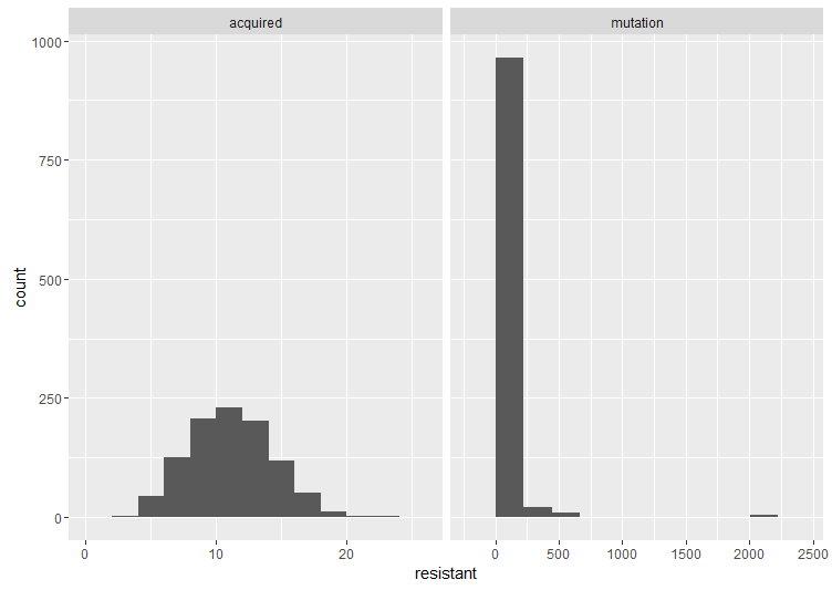
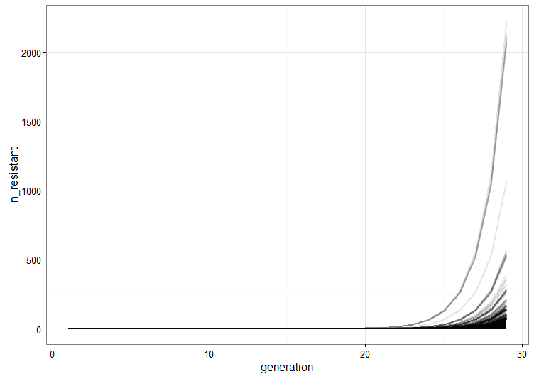
, which is quite close to their estimated value, and that the mutation can’t reverse. We also assume that the bacteria grow by doubling each generation up to 30 generations. We start a culture from a single susceptible bacterium, and let it grow for a number of generations before the phage is added. (We’re going to use discrete generations, while Luria & Delbrück use a continuous function.) Then:

n_{susceptible,i+1}= 2 (n_{susceptible,i} - n_{mutants,i})

n_{resistant,i+1} = 2 (n_{resistant,i} + n_{mutants,i})

That is, every generation i, the mutants that occur move from the susceptible to the resistant category. The number of mutants that happen among the susceptible is binomially distributed:

n_{mutants,i} \sim Binomial(n_{susceptible,i}, \mu) .

This is an R function to simulate a culture:

culture <- function(generations, mu) {
  n_susceptible <- numeric(generations)
  n_resistant <- numeric(generations)
  n_mutants <- numeric(generations)
  n_susceptible[1] <- 1
  for (i in 1:(generations - 1)) {
    n_mutants[i] <- rbinom(n = 1, size = n_susceptible[i], prob = mu)
    n_susceptible[i + 1] &lt;- 2 * (n_susceptible[i] - n_mutants[i])
    n_resistant[i + 1] &lt;- 2 * (n_resistant[i] + n_mutants[i])
  }
  data.frame(generation = 1:generations,
             n_susceptible,
             n_resistant,
             n_mutants)
}
cultures <- replicate(1000, culture(30, 2e-8), simplify = FALSE)

We run a few replicate cultures and plot the number of resistant bacteria. This graph shows the point pretty well: Because of random mutation and exponential growth, the cultures where mutations happen to arise relatively early will give rise to a lot more resistant bacteria than the ones were the first mutations are late. Therefore, there will be a lot of variation between the cultures because of their different histories.

resistant

combined <- Reduce(function (x, y) rbind(x, y), cultures)
combined$culture <- rep(1:1000, each = 30)

resistant_plot <- qplot(x = generation, y = n_resistant, group = culture,
      data = combined, geom = "line", alpha = I(1/10), size = I(1)) + theme_bw()

We compare this to what happens under the alternative hypothesis where resistance arises as a consequence of introduction of the phage with some resistance rate (this is not the same as the mutation rate above, even though we’re using the same value). Then the number of resistant cells in a culture will be: n_{acquired} \sim Binomial(2^{29}, \mu_{aquried}) .

resistant <- unlist(lapply(cultures, function(x) max(x$n_resistant)))

acquired_resistant <- rbinom(n = 1000, size = 2^29, 2e-8)

resistant_combined <- rbind(transform(data.frame(resistant = acquired_resistant), model = "acquired"),
                            transform(data.frame(resistant = resistant), model = "mutation"))

resistant_histograms <- qplot(x = resistant, data = resistant_combined,bins = 10) +
  facet_wrap(~ model, scale = "free_x")

histograms

Here are two histograms side by side to compare the cases. The important thing is the shape. If the acquired resistance hypothesis holds, the number of resistant bacteria in replicate cultures follows a Poisson distribution, because it arises when one counts the number of binomially distributed events that occur in a given number of trials. The interesting thing about the Poisson distribution in this case is that its mean is equal to the variance. However, under the mutation model (as we’ve already illustrated), there is a lot of variation between cultures. These fluctuations make the variance much larger than the mean, which is also what Luria and Delbrück found in their data. Therefore, the results are inconsistent with acquired mutation, and hence the experiment is called the Luria–Delbrück fluctuation test.

mean(resistant)
var(resistant)
mean(acquired_resistant)
var(acquired_resistant)

Literature

Luria, S. E., & Delbrück, M. (1943). Mutations of bacteria from virus sensitivity to virus resistance. Genetics, 28(6), 491.

Meneely, P. M. (2016). Pick Your Poisson: An Educational Primer for Luria and Delbrück’s Classic Paper. Genetics, 202(2), 371-375.

Code on github.

På dna-dagen: Gener, orsak och verkan

”DNA, livets molekyl” … Visst, DNA är en viktig och snygg biomolekyl. Men varför skulle inte en komplex kolhydrat, ett protein eller en membranlipid förtjäna det namnet?

Det finns två perspektiv på genetik som jag brukar tjata om. Å ena sidan: genetik som handlar om vad molekylära gener gör och vad de har för funktion. Å andra sidan: genetik som är studiet av ärftliga skillnader mellan individer, och i förlängningen populationer och arter. Genetik beskrivs ibland som en vetenskap som handlar om ”koder” och ”information”. Det ligger något i det, men jag tror det är bra att vara lite försiktig med metaforerna. Jag misstänker att koder och information inte är något vi bara hittar liggande ute i naturen, så att säga, utan mänskliga tolkningar.

Ja, vissa DNA-sekvenser skrivs av till mRNA som kodar för proteiner. Här betyder ”kodar för” att sekvensen har tripletter av baser som är komplementära mot tRNA-molekyler som bär aminosyror. Andra sekvenser motsvarar RNA-molekyler som har någon annan funktion. Men de orsakande faktorerna till att ett visst RNA uttrycks vid en viss tid finns inte i DNA, utan någon annan stans. DNA är en del av mekanismen, men det är också RNA-polymeraset som skriver av det, spliceosomen som sätter ihop aktivt mRNA, de system av enzymer som tillverkar nukleotiderna och så vidare, och så vidare. Processen aktiveras av vad som händer i organismens miljö, interna processer som omfattar många delar av cellen eller helt olika delar av kroppen osv. På så sätt är kärnan med sitt DNA en organell vilken som helst.

Men! Det finns ett sammanhang där det är befogat att prata om genetiska orsaker, nämligen ärftliga skillnader mellan individer. Det går att hitta (och faktiskt konstruera) exempel på individer där dramatiska skillnader i egenskaper som utseende och beteende beror på en skillnad i DNA-sekvens — en genetisk variant eller ”gen” i den klassiska bemärkelsen. Det förstås, det kan finnas andra typer av ärftlighet som inte beror på DNA, och i så fall borde de också räknas med här. Men de flesta saker som inuti celler kan göra skillnad i en organisms egenskaper — proteiner, membranlipider, kolhydrater, små organiska molekyler osv — nollställs mellan generationerna, när könsceller bildas och utvecklingen så att säga börjar om varje generation. Men DNA går i arv — med sin ”information”, om en så vill.

(Den 25 april 1953 publicerades artiklarna som presenterade DNA-molekylens struktur. Därav DNA-dagen. Min DNA-dagspost från förra året: På dna-dagen)

Paper: ”Mixed ancestry and admixture in Kauai’s feral chickens: invasion of domestic genes into ancient Red Junglefowl reservoirs”

We have a new paper almost out (now in early view) in Molecular Ecology about the chickens on the Pacific island Kauai. These chickens are pretty famous for being everywhere on the island. Where do they come from? If you use your favourite search engine you’ll find an explanation with two possible origins: ancient wild birds brought over by the Polynesians and escaped domestic chickens. This post on Kauaiblog is great:

Hawaii’s official State bird is the Hawaiian Goose, or Nene, but on Kauai, everyone jokes that the “official” birds of the Garden Island are feral chickens, especially the wild roosters.

Wikepedia says the “mua” or red jungle fowl were brought to Kauai by the Polynesians as a source of food, thriving on an island where they have no real predators. /…/
Most locals agree that wild chickens proliferated after Hurricane Iniki ripped across Kauai in 1992, destroying chicken coops and releasing domesticated hens, and well as roosters being bred for cockfighting. Now these brilliantly feathered fowl inhabit every part of this tropical paradise, crowing at all hours of the day and night to the delight or dismay of tourists and locals alike.

In this paper, we look at phenotypes and genetics and find that this dual origin explanation is probably true.

jeff_trimble_kauai_chickens_cc_by_nc_sa

(Chickens on Kauai. This is not from our paper, but by Jeff Trimble (cc:by-sa-nc) published on Flickr. There are so many pretty chicken pictures there!)

Dom, Eben, and Pamela went to Kauai to photograph, record to and collect DNA from the chickens. (I stayed at home and did sequence bioinformatics.) The Kauai chickens look and sound like mixture of wild and domestic chickens. Some of them have the typical Junglefowl plumage, and other have flecks of white. Their crows vary in the length of the characteristic fourth syllable. Also, some of them have yellow legs, a trait that domestic chickens seem to have gotten not from the Red but from the Grey Junglefowl.

We looked at DNA sequences by massively parallel (SOLiD) sequencing of 23 individuals. We find mitochondrial sequences that fall in two haplogroups: E and D. The presence of the D haplogroup, which is the dominating one in ancient DNA sequences from the Pacific, means that there is a Pacific component to their ancestry. The E group, on the other hand, occurs in domestic chickens. It also shows up in some ancient DNA samples from the Pacific, but not from Kauai (and there is a scientific debate about these sequences). The nuclear genome analysis is pretty inconclusive. I think what we would need is some samples of possible domestic source populations (Where did the escapee  chickens came from? Are there other traditional domestic sources?) and a better sampling of Red Junglefowl to make better sense of it.

When we take the plumage, vocalisation and mitochondrial DNA together, it looks like this is a feral admixed population of either Red Junglefowl or traditional Pacific chickens mixed with domestics. A very interesting population indeed.

Kenneth Chang wrote about the paper in New York Times; includes quotes from Eben and Dom.

E Gering, M Johnsson, P Willis, T Getty, D Wright (2015) Mixed ancestry and admixture in Kauai’s feral chickens: invasion of domestic genes into ancient Red Junglefowl reservoirs. Molecular ecology

Morning coffee: cost per genome

I recently heard this thing referred to as ”the most overused slide in genomics” (David Klevebring). It might be: what it shows is some estimate of the cost of sequencing a human genome over time, and how it plummets around 2008. Before that, the curve is Sanger sequencing, and then the costs show second generation sequencing (454, Illumina and SOLiD).

cost_genome

The source is the US National Human Genome Research Institute, and they’ve put some thought into how to estimate costs so that machines, reagents, analysis and people to do the work are included and that the different platforms are somewhat comparable. One must first point out that downstream analysis to make any sense of the data (assembly and variant calling) isn’t included. But the most important thing that this graph hides, even if the estimates of the cost would be perfect, is that to ”sequence a genome” means something completely different in 2001 and 2015. (Well, with third generation sequencers that give long reads coming up, the old meaning might come back.)

For data since January 2008 (representing data generated using ‘second-generation’ sequencing platforms), the ”Cost per Genome” graph reflects projects involving the ‘re-sequencing’ of the human genome, where an available reference human genome sequence is available to serve as a backbone for downstream data analyses.

The human genome project was of course about sequencing and assembling the genome into high quality sequences. Very few of the millions of human genomes resequenced since are anywhere close. As people in the sequencing loop know, resequencing with short reads doesn’t give you a genome sequence (and neither does trying to assemble a messy eukaryote genome with short reads only). It gives you a list of variants compared to the reference sequence. The usual short read business has no way of detect anything but single nucleotide variants and small indels. (And the latter depends … Also, you can detect copy number variants, but large scale structural variants are mostly off the table.) Of course, you can use these edits to reconstruct a consensus sequence from the reference, but it would be a total lie.

Again, none of this is news for people who deal with sequencing, and I’m not knocking second-generation sequencing. It’s very useful and has made a lot of new things possible. It’s just something I think about every time I see that slide.

Interaktioner mellan gener förklarar antagligen inte den saknade ärftligheten

Har fått flera tips om den här artikeln:

Asko Mäki-Tanila & William Hill (2014)  Influence of Gene Interaction on Complex Trait Variation with Multilocus Models. Genetics.

Den har en hyfsat torr titel och rätt många ekvationer och handlar om något av det intressantaste nämligen kvantitativa egenskaper och gen–gen-interaktioner. Saknad heritabilitet är ett känt genetiskt problem. Det finns flera förslag på lösningar och det är bara att välja sin favorit. Författarnas beräkningar tyder på att den antagligen inte förklaras av interaktioner mellan gener. (Varning: ganska lång och nördig bloggpost. Som vanligt.)

Vad är heritabilitet? Vi tänker oss en egenskap som varierar i en population. Om egenskapen är ärftlig kommer en del av variationen att gå i familjen. Och om vi mäter den och har ett släktträd över individerna kan vi uppskatta hur stor del av variationen som förklaras av släktskap. Detta uttrycks som varianser och kvoten mellan additiv genetisk varians och den totala variansen kallas heritabilitet. (Vadå ”additiv”? Vi kommer tillbaka till det.) Heritabiliteten är ett bråktal mellan noll och ett där ett större värde är en större ärftlig komponent.

Vad är det som saknas? Vi ska inte göra någon katalog, men det finns otaliga olika egenskaper hos växter och djur som är delvis ärftliga. Många har också gjort genetisk kartläggning (en samling tekniker som jag ofta tjatar om, bara delvis för att jag jobbar med dem) för att hitta de gener som förklarar ärftligheten och kunna undersöka hur de fungerar. Problemet är att de gener som går att hitta nästan alltid bara förklarar en liten andel av den ärftliga variationen. För nästan alla egenskaper finns det en avsevärd ”saknad heritabilitet” som måste bero på okända genetiska varianter. Den saknade delen är nästan alltid mycket större än den som förklaras av kända varianter. Exempel: Nyligen publicerades en analys av mänsklig längd baserad på 250 000 individer (Wood & al 2014). Den hittar cirka 700 genetiska varianter som tillsammans förklarar ungefär en femtedel av heritabiliteten.

Okej, så var gömmer den sig? Förmodligen är det är många varianter som bidrar med mycket små enskilda effekter. Då skulle det behövas ännu större studier för att hitta dem. I vissa egenskaper kanske det också är frågan om ovanliga varianter som bara finns i vissa familjer. I så fall skulle de inte hittas i stora populationsstudier utan drunkna i bruset. Men det finns också mer exotiska hypoteser om den saknade heritabiliteten. En är att det skulle vara epigenetisk variation snarare än genetisk (varför jag inte tror det är förklaringen borde jag skriva mer om någon annan gång). En annan är gen–gen-interaktioner, eller på genetiskt fikonspråk epistasi.

Dags att återvända till den additiva genetiska variansen. Det kan nämligen finnas en genetisk komponent som inte direkt går i arv från föräldrar till avkomma. Anlagen går i arv, naturligtvis, men avkommans egenskaper kan bli helt annorlunda om det finns interaktioner mellan olika genetiska varianter. Det blir tydligast med ett exempel med en egenskap som kan delas in i tydliga kategorier och som styrs av varianter på två gener. Det här är ett exempel från världens bästa organism, nämligen hönan.

Titta på bilden. Panel A: en vanlig enkel hönskam. Panel C: pärlkam som orsakas av en genreglerande variant i genen SOX5 (Wright & al 2009). Panel B: rosenkam, som orsakas av omflyttning som påverkar regleringen av genen NMR2 (Imsland & al 2012). Panel D: valnötskam, vilket är vad som händer de som bär båda mutationern. SOX5 och NMR2 är aktiva i samma cellpopulation i förstadiet till kammen under embroynalutvecklingen. Interaktionen mellan varianter som påverkar SOX5 och NMR2 beror förmodligen på att de ingår samma system som bygger upp kammen.

kammar_imsland

(Figur 1 från Imsland & co 2012. cc:by-3.0)

Nu är de flesta intressanta egenskaper inte så enkla och kategoriska som kamtyperna. Principen är ändå densamma. Effekten av en genetisk variant kan bero på vilka andra varianter individen bär på. Detta kallas epistasi.

Det Mäki-Tanilas & Hill tittat närmare på är vad som händer på populationsnivå. De utgår från en hyfsat realistisk situation, det finns ett antal genetiska varianter på olika gener, som alla påverkar samma egenskap. Om varianterna dessutom interagerar med varandra, vad händer med den genetiska variansen? Är den fortfarande huvudsakligen additiv, alltså sådan som går i arv från föräldrar till avkomma, eller blir det en stor icke-additv genetisk varianskomponent istället? På det hela taget så blir det oftast mest additiv genetisk varians, även om det finns interaktioner mellan varianterna.

Varför? Om vi tittar på undantagen: Interaktioner blir märkbara på populationsnivå när det är få varianter som påverkar en egenskap eller när varianterna är vanliga i populationen. Om det är många gener som påverkar egenskapen så späs interaktioneffekterna ut, men epistasi kan ha stor effekt på egenskaper med relativt enkel genetik och få gener. Sådana egenskaper verkar inte vara så vanliga, men de kan finnas. Om en av allelerna (de räknade bara på bara fallet med två alleler per gen) är ovanlig betyder det också att epistasi spelar mindre roll. Om de flesta indiver är genetiskt lika kommer det vara väldigt ovanligt att samma individ bär på flera av varianterna som krävs för att interaktionseffekten ska märkas.

Ta ett helt hypotetiskt exempel: Gen 1 har två varianter stora A och lilla a. Gen 2 ha två varianter stora B och lilla b. Varianten A gör dig i medeltal 1 mm längre. B gör dig också i medeltal 1 mm längre. Men om du råkar ha både A och B får du en extra skjuts på 2 mm, förutom den sammanlagda effekten. Men om populationens genpool nästan helt domineras av a på Gen 1 och b på Gen 2 så kommer individer med både A och B vara väldigt ovanliga. De har ingen större effekt på längdfördelningen i populationen, sådär i allmänhet. Men de gör att enskilda individer med ovanliga genotyper blir ovanligt långa.

Så, författarna hävdar att interaktioner antagligen inte förklarar den saknade heritabiliteten. Tidigare har Zuk m.fl (Zuk & al 2012) föreslagit att en förklaring skulle kunna vara att interaktioner mellan gener stör skattningen av heritabilitet. Mäki-Tanilas & Hills modell tyder på att egenskaper beter sig additivt i alla fall, så det är okej att ignorera interaktioner i heritabilitetsmätningar. Vem som har rätt beror på vilken modell som stämmer bäst med hur komplexa ärftliga egenskaper egentligen fungerar. Jag är böjd att tro att det är den senare modellen, men är inte helt säker.

Det finns en sorts motsättning om epistasi. Å ena sidan verkar egenskaper ha mycket additiv varians. Å andra sidan går det att hitta mängder av interaktioner på molekylär nivå. Gener borde interagera. Om Mäki-Tanila & Hill har rätt så har de förklaringen: det är mycket möjligt att det finns massor av epistasi, men under de vanliga förhållanden är den dominerande varianskomponenten ändå den additiva. Vi som gillar interaktioner kan äta kakan och ha den kvar.

Interaktioner är fortfarande intressanta. För att kunna förutsäga en individs egenskaper från dess genotyper behövs information om hur varianter interagerar med varandra. Det är möjligt att epistasi visar sig vara vanligt i komplexa egenskaper (som en del misstänker). Problemet är att det är så svårt att studera. Att söka efter interagerande par av gener är rutin i vissa typer av kartläggning (som de experimentkorsningar jag sysslar med) men svårare i helgenomsassociation. Jag tror inte det är någon som vet riktigt hur det ska gå till.

Finding the distance from ChIP signals to genes

I’ve had a couple of months off from blogging. Time for some computer-assisted biology! Robert Griffin asks on Stack Exchange about finding the distance between HP1 binding sites and genes in Drosophila melanogaster.  We can get a rough idea with some public chromatin immunoprecipitation data, R and the wonderful BEDTools.

Finding some binding sites

There are indeed some ChIP-seq datasets on HP1 available. I looked up these ones from modENCODE: modENCODE_3391 and modENCODE_3392, using two different antibodies for Hp1b in 16-24 h old embroys. I’m not sure since the modENCODE site doesn’t seem to link datasets to publications, but I think this is the paper where the results are reported: A cis-regulatory map of the Drosophila genome (Nègre & al 2011).

What they’ve done, in short, is cross-linking with formaldehyde, sonicate DNA into fragments, capture fragments with either of the two antibodies and sequence those fragments. They aligned reads with Eland (Illumina’s old proprietary aligner) and called peaks (i.e. regions where there is a lot of reads, which should reflect regions bound by Hp1b) with MACS. We can download their peaks in general feature format.

I don’t know whether there is any way to make completely computation predictions of Hp1 binding sites but I doubt it.

Some data cleaning

The files are available from ftp, and for the below analysis I’ve unzipped them and called them modENCODE_3391.gff3 and modENCODE_3392.gff3. GFF is one of all those tab separated text files that people use for genomic coordinates. If you do any bioinformatics type work you will have to convert back and forth between them and I suggest bookmarking the UCSC Genome Browser Format FAQ.

Even when we trust in their analysis, some processing of files is always required. In this case, MACS sometimes outputs peaks with negative start coordinates in the beginning of a chromosome. BEDTools will have none of that, because ”malformed GFF entry at line … Start was greater than end”. In this case, it happens only at a few lines, and I decided to set those start coordinates to 1 instead.

We need a small script to solve that. As I’ve written before, any language will do, but I like R and tend to do my utility scripting in R (and bash). If the files were incredibly huge and didn’t fit in memory, we’d have to work through the files line by line or chunk by chunk. But in this case we can just read everything at once and operate on it with vectorised R commands, and then write the table again.

modENCODE_3391 <- read.table("modENCODE_3391.gff3", stringsAsFactors=F, sep="\t")
modENCODE_3392 <- read.table("modENCODE_3392.gff3", stringsAsFactors=F, sep="\t")

fix.coord <- function(gff) {
  gff$V4[which(gff$V4 < 1)] <- 1
  gff
}

write.gff <- function(gff, file) {
  write.table(gff, file=file, row.names=F, col.names=F,
              quote=F, sep="\t")
}

write.gff(fix.coord(modENCODE_3391), file="cleaned_3391.gff3")
write.gff(fix.coord(modENCODE_3392), file="cleaned_3392.gff3")

Flybase transcripts

To find the distance to genes, we need to know where the genes are. The best source is probably the annotation made by Flybase, which I downloaded from the Ensembl ftp in General transfer format (GTF, which is close enough to GFF that we don’t have to care about the differences right now).

This file contains a lot of different features. We extract the transcripts and find where the transcript model starts, taking into account whether the transcript is in the forward or reverse direction (this information is stored in columns 4, 5 and 7 of the GTF file). We store this in a new GTF file of transcript start positions, which is the one we will feed to BEDTools:

ensembl <- read.table("Drosophila_melanogaster.BDGP5.75.gtf",
                      stringsAsFactors=F, sep="\t")

transcript <- subset(ensembl, V3=="transcript")
transcript.start <- transcript
transcript.start$V3 <- "transcript_start"
transcript.start$V4 <- transcript.start$V5 <- ifelse(transcript.start$V7 == "+",
                                                     transcript$V4, transcript$V5)

write.gff(transcript.start, file="ensembl_transcript_start.gtf")

Finding distance with BEDTools

Time to find the closest feature to each transcript start! You could do this in R with GenomicRanges, but I like BEDTools. It’s a command line tool, and if you haven’t already you will need to download and compile it, which I recall being painless.

bedtools closest is the command that finds, for each feature in one file, the closest feature in the other file. The -a and -b flags tells BEDTools which files to operate on, and the -d flag that we also want it to output the distance. BEDTools writes output to standard out, so we use ”>” to capture it in a text file.

Here is the bash script. I put the above R code in clean_files.R and added it as an Rscript line at the beginning, so I could run it all with one file.

#!/bin/bash
Rscript clean_files.R

bedtools closest -d -a ensembl_transcript_start.gtf -b cleaned_3391.gff3 \
    > closest_element_3391.txt
bedtools closest -d -a ensembl_transcript_start.gtf -b cleaned_3392.gff3 \
    > closest_element_3392.txt

Some results

With the resulting file we can go back to R and ggplot2 and draw cute graphs like this, which shows the distribution of distances from transcript to Hp1b peak for protein coding and noncoding transcripts separately. Note the different y-scales (there are way more protein coding genes in the annotation) and the 10-logarithm plus one transformation on the x-axis. The plus one is to show the zeroes; BEDTools returns a distance of 0 for transcripts that overlap a Hp1b site.

closest_3391 <- read.table("~/blogg/dmel_hp1/closest_element_3391.txt", header=F, sep="\t")

library(ggplot2)
qplot(x=log10(V19 + 1), data=subset(closest_3391, V2 %in% c("protein_coding", "ncRNA"))) +
  facet_wrap(~V2, scale="free_y")

distance_hist

Or by merging the datasets from different antibodies, we can draw this strange beauty, which pretty much tells us that the antibodies do not give the same result in terms of the closest feature. To figure out how they differ, one would have to look more closely into the genomic distribution of the peaks.

closest_3392 <- read.table("~/blogg/dmel_hp1/closest_element_3392.txt", header=F, sep="\t")

combined <- merge(closest_3391, closest_3392,
                  by.x=c("V1", "V2","V4", "V5", "V9"),
                  by.y=c("V1", "V2","V4", "V5", "V9"))

qplot(x=log10(V19.x+1), y=log10(V19.y+1), data=combined)

between_antibodies

(If you’re wondering about the points that end up below 0, those are transcripts where there are no peaks called on that chromosome in one of the datasets. BEDTools returns -1 for those that lack matching features on the same chromosome and R will helpfully transform them to -Inf.)

About the DGRP

The question mentioned the DGRP. I don’t know that anyone has looked at ChIP in the DGRP lines, but wouldn’t that be fun? Quantitative genetics of DNA binding protein variation in DGRP and integration with eQTL … What one could do already, though, is take the interesting sites of Hp1 binding and overlap them with the genetic variants of the DGRP lines. I don’t know if that would tell you much — does anyone know what kind of variant would affect Hp1 binding?

Happy hacking!

Journal club of one: ”Genome-wide association of foraging behavior in Drosophila melanogaster fails to support large-effect alleles at the foraging gene” (preprint)

This preprint was posted on bioRxiv and Haldane’s sieve. It tells the story of one of the best known genetic variants affecting behaviour, the foraging gene in Drosophila melanogaster. for is still a nice example of a large-effect variant causing (developmentally) pleiotropic effects. However, Turner & al present evidence questioning whether for has any substantial effect in natural populations of flies. I think it’s self-evident why I’m interested.

They look at previous evidence for foraging as a quantitative trait gene in files sampled from natural populations and perform genome-wide association and population genetic tests with 35 DGRP lines, finding nothing at the for locus.

Comments:

(Since this is a preprint, I will feel free to suggest what I think could be improvements to the manuscript. Obviously, these are just my opinions.)

I’m not convinced one can really separate a unimodal from a bimodal distribution with 36 data points? Below are a few histograms simulated from a mixture of two normal distributions where 25 samples are ”rovers” and 11 ”sitters”.

bimodal

For fun, I also tested for normality with the Shapiro-Wilks’ test as the authors did, and about half of 1000 tests reject. My histograms should not be overinterpreted; I just generated two normal distributions with means log10(2.66) and log10(1.3) with standard deviations 0.1. I don’t know the actual standard deviations of the forS and forR reference strains. Of course, when the standard deviation is small enough, the distributions clearly separate and Shapiro-Wilks’ test will reject.

Power is difficult, but in this case the authors are looking at a well-known effect. They should be able to postulate some reasonable effect-sizes given the literature and the difference between the reference strains and make sure that they’re actually powered to detect it. 35 individuals for a GWAS is not much. They may still have good power to detect a effect of the size expected at for, at least in the single-point test, but it would be nice to demonstrate it. Power feels particularly pertinent as the authors claim to find evidence of absence. The same thing should apply to the population genetic tests, though it’s probably harder to know what effects to expect there.

The authors discuss alternative interpretations, and mention  the fact that in their hands the reference strains did not travel nearly as long as in previous experiments. How likely is it, though, that the variant isn’t segregating in Raleigh but in the populations previously sampled?

Literature

Thomas Turner, Christopher C Giauque, Daniel R Schrider, Andrew D Kern. (2014) Genome-wide association of foraging behavior in Drosophila melanogaster fails to support large-effect alleles at the foraging gene. Preprint on bioaRxiv. doi: 10.1101/004325